2. First look into particle simulations¶

Learning goals:

To learn the basic terms and terminology of particle simulations
To have a basic understanding of molecular topologies
To understand the difference between particle and continuum models
To understand the concept of force field

Keywords: Particle simulations, molecular dynamics, Monte Carlo, continuum simulations, molecular topology, force field, interactions

Note: The links are provided for additional information for those interested, not as required reading.

It is finally the time to discuss some of the basic concepts of particle simulations. As this is the first description, it does not aim to be complete, but rather practical in the sense that basic concepts and terminology are introduced. This information will be needed and elaborated later and this knowledge will help in setting up simulations and in data analysis.

2.1. Particle vs continuum simulations¶

Although particle simulations seems almost too obvious a term, it needs some attention. The most common basic object in a particle simulation is an atom or, rather, a generalized atom. In this course we are mostly dealing with atoms in the sense that they don’t have electrons. Their overall averaged properties are included in the force fields as we will discuss.

Force field: The parameters and functions that describe interactions in simulations.

These electron-less atoms do, however, have many other properties allowing for comparisons between the simulation results and experiments as long as one is in the same atomistic scales (for example energies, diffusion coefficients and such). The important concept here is that by particle simulations we refer to a system which is composed of discrete entities.

Atom: From the Greek word atomos, which means "uncuttable".

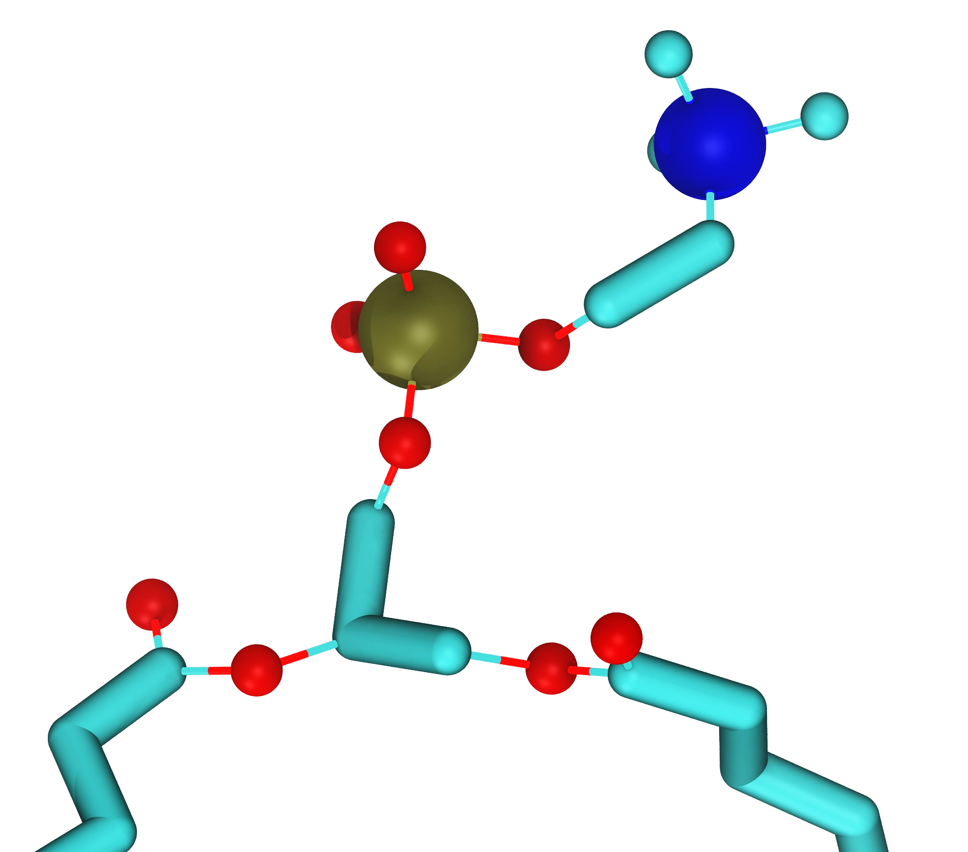
These discrete entities may also be coarse-grained atoms (sometimes also called superatoms). The concept of a coarse-grained atom can be thought of as follows: Assume that there is some method that allows us to average over some chosen physical properties of a group of atoms, for example a group of atoms in a polymer, and combine them to a single larger entity. That new entity is then a coarse-grained atom. At first sight such a procedure may sound like that may sound like heresy or nonsense, but there are some well-justified and rigorous methods for such procedures. Such methods will not be discusses here but in case interested, see for example references[7][2]. An example of such an approach is the so-called MARTINI force field[5] in which four ‘atomistic’ atoms are a coarse-grained into one larger unit.

Fig. 2.9 Examples of coarse graining. Left: A single water molecule with its hydrogens and oxygens coarse grained to a single new coarse-grained water. Right: Four water molecules coarse-grained to a single coarse-grained water molecule. This approach is used in the very popular MARTINI model[5]. Note that the size of a water molecule is about 2.8 Å.¶

Simulations of even large non-atomistic entities such as planets are in the category of particle simulations since they are discrete entities. In such simulations, the internal structure of planets or celestial bodies is not included in the simulated properties. This is similar in spirit to not taking electrons into account in atomic-level molecular dynamics simulations. Other examples that may not be so obvious at first sight are entities such as lattice defects in solid state systems. Defects can be treated as discrete entities and they have properties such as size and they interact over distances. Here, we use ‘atomistic’ atoms and the term atomistic is used for describing systems at the atomic scale of Ångströms and nanometers.

Fig. 2.10 Two examples of a lattice. Left: A hexagonal lattice with one lattice site highlighted in red. The nearest neighbors (6) of the site are marked in blue. Middle: A square lattice. The nearest neighbors (4) of a selected site (red) are marked in blue. When simulating continuum models, the partial differential equations are solved using finite difference methods on a lattice. Thus, the space is not continuous like in a particle simulation (right).¶

In contrast to particle simulations, in continuum modeling one often uses a fixed underlying lattice or grid in which one solves finite difference equations. In such simulations the material (say, a liquid, gas or a solid) is described by a continuous field instead of an atom. This means that, unlike in an atomistic simulations, the material no longer has internal structure but it is described by a field or several fields. The field(s) is (are) placed on a discrete grid and the evolution of the field(s) is (are) solved on a computer; the corresponding equations of motion are solved on a lattice or using finite element methods (FEM). Such approaches are commonly used in the fields of materials research and reaction-diffusion systems.

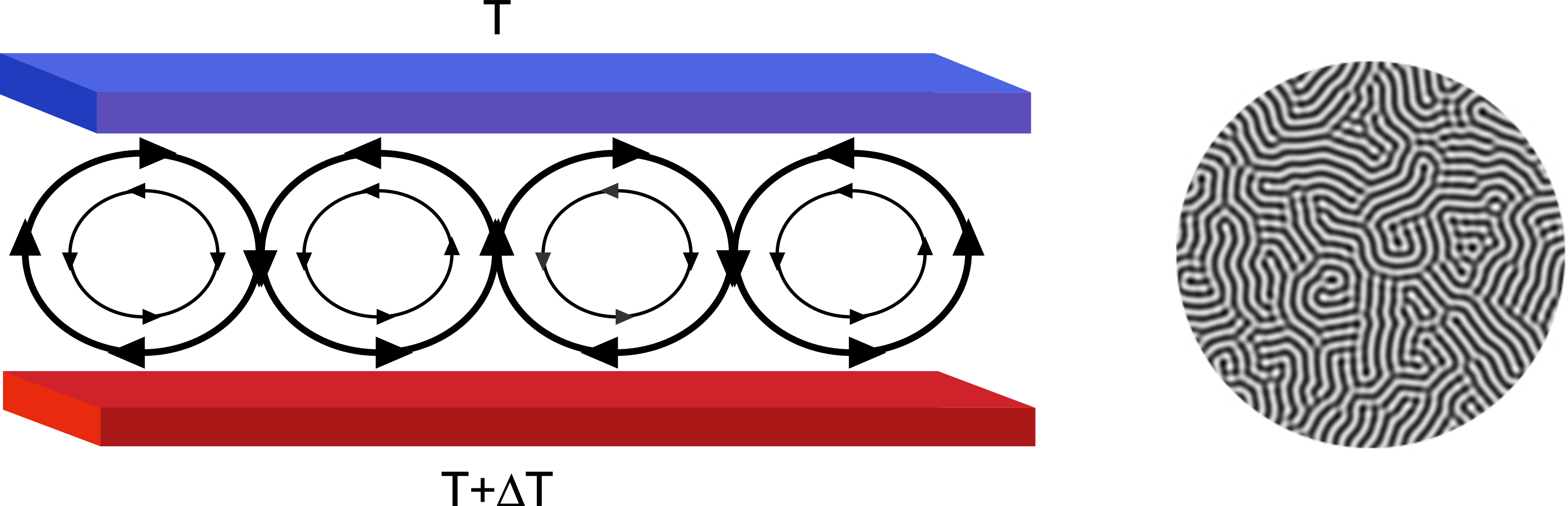
Fig. 2.11 Example of continuum modeling. Assume a situation in which fluid is placed between two plates. The lower plate is kept at a higher temperature than the upper one (left). As the warmer and lighter fluid raises to the top, the top layer cools and becomes denser and heavier. This can lead to rotation of water as indicated by the arrows: the heavier fluid drops and lighter rises. The picture on the right shows a top view of such a situation using continuum modeling (phase-field model). Model this type of a system would require too many particles and hence one has to use continuum models. In this case, the equations of motion (partial differential equations) were solved on a square lattice. This type of physical situation occurs, for example in oceans and is called Rayleigh-Benard convection.¶

2.2. Simulation methods for particle systems¶

The main simulation methods for particle systems are Monte Carlo and Molecular Dynamics (MD).

2.2.1. Monte Carlo¶

In this course the focus is on the molecular dynamics method, but for completeness, let’s briefly discuss the Monte Carlo (MC) method since it is one the most widely used simulation techniques (if not the most widely used) with applications ranging from social sciences, to optimizing public transport networks to particle simulations.

The MC method does not solve any equations of motion, instead it is a stochastic optimization method using an energy function: No time integration is involved but one uses random numbers for optimizing selected properties. In the case molecular systems, one typically optimizes (minimizes) the potential energy. This also means that, in its basic form, MC cannot measure any dynamical properties (there are variants like the kinetic Monte Carlo but even that doesn’t have time integration). Instead, MC uses ensemble averaging to compute the system’s properties.

The basic idea of MC simulation is that it uses pseudo-random numbers to overcome local energy barriers to reach the minimum energy state. Random numbers are used to give the system a small probability to move in the direction that is energetically unfavorable. That is, in a crude sense the system ‘gambles’ to find the global minimum state; the name Monte Carlo comes from the Monte Carlo Casino in the city of Monaco in Southern France. In terms of an atomistic system, only the positions of the atoms are used and there are no velocities. Since the particles have mutual interactions described by a potential energy, minimization of potential energy yields the equilibrium configuration of the system. The part that sometimes causes confusion is that in MC, term Monte Carlo steps is used. The term indicates the number of so-called Monte Carlo sweeps and it is sometimes falsely equated to the time steps in MD simulations. In MD, there is a real time step (typically in terms of femtoseconds) but the MC step does not correspond to any physical time.

Fig. 2.12 The concept behind the Monte Carlo method. Consider that a system’s state is described the green sphere and the that the energy landscape is given by the dashed line. Deterministic optimization finds the closest minimum as indicated by the arrow in the left hand side figure. Once the minimum has been reached, the system stays there. Monte Carlo is a stochastic optimization method. It uses random numbers to enable the system to move uphill in the energetically unfavorable direction as indicated by the arrow in the right hand side figure. Once the system crosses the saddle point, it can find the global minimum.¶

Technically, a Monte Carlo simulation is the evaluation of statistical mechanical configuration integral and we will discuss this point later and it generates representative samples of the system.The key ingredients are the application of a probability distribution and the use of random numbers. In the case of physical systems, the equilibrium state has a unique distribution: the Boltzmann distribution.

Although it may not be clear from the above, one of the great advantages of the MC method is its flexibility. In terms of atoms or particles, it can be used to simulate classical and quantum mechanical systems. It can also be applied to systems of very different nature such as optimizing train scheduling for railway networks and to numerically solve complex mathematical integrals that have no analytical solution.

2.2.2. Classical Molecular Dynamics¶

Now that we have an idea of the Monte Carlo, let’s move on to our main interest, the MD method. We can define classical Molecular Dynamics the following way:

Definition of Molecular Dynamics (MD)

Molecular Dynamics is the evolution of Newton’s equations motion in time.

This definition has several important points:

We have a dynamical system that evolves in time. That is, it provides time-resolved information. This is in contrast to the Monte Carlo method.
The evolution of the system in the phase space is determined by solving Newton’s equations of motion for all the particles that comprise the system.
In the absence of external forces and fields, the system must evolve toward equilibrium, that is, the state of minimum free energy. Statistical mechanics tells us that equilibrium described by a unique distribution, the Boltzmann distribution.

The first published article using classical MD simulations titled “Phase Transition for a Hard Sphere System” was published by Alder and Wainwright in 1957[1]. They simulated systems of 32 hard particles and also shorter simulations with 108 particles. As already discussed, the first MC simulations were performed a few years before in 1952 by Metropolis et al.[2]. Other landmarks include the paper of Gibson et al., “Dynamics of Radiation Damage” which is the first time for using continuous potentials in an MD simulation the same spirit as we do today[3]. Another interesting point is the number of time steps taken in their simulation. They had 500 atoms and reported a total 219 steps which took over 3.5 hours. Keep this number in mind for the time when we set up our own simulations. Another landmark in MD simulations is the emergence of force fields and the first QM/MM simulations which can be traced to the articles of Warshel, Karplus and Lifson in the late 1960’s and early 1970s[4][10].

2.2.3. What is the output of a particle simulation?¶

The basic result of a particle simulation is a trajectory, that is, the positions of atoms written at a requested output interval (the output interval is typically given as an input parameter for the simulation). In the case of an MD simulation, it is also possible to output the velocities and forces together with the positions. MC simulation, however, does not have velocities or forces. Instead, it has energies. They can be written out at the the requested interval. One should also notice that whereas MD simulation has time and output interval is given in terms of time (or steps that can be easily converted to time), in a Monte Carlo simulation the MC step has no relation to real time.

Most simulations programs also output other quantities such as energies, pressures, the size of the simulation box and so on. However, the trajectory is the most fundamental outcome of a particle simulation and it is the basis of more detailed analyses.

Example output from an MD simulation

The actual output format varies depends on the software, but in the most typical case positions of all atoms are stored. It is also possible to store velocities and forces in the case of MD simulations. The example below shows an output in the format of Gromacs .gro file.

The output below has been extracted (5 water molecules out of 216 were selected) from the file spc216.gro that comes with Gromacs; the full file will be used when we set up simulations that include water. Notice also that most software, including Gromacs can output trajectory data in multiple formats. The example below is the human-readable .gro format but during a simulation binary formats are used since they take much less space to store. File formats will be discussed in detail in later lectures.

The 1st line has comments. Arbitrary information can be included and this line is ignored by analysis software. In this case is says: 5 water molecules, SPC model, temperature of 300K and box size of 1.86206.
The 2nd line: The total number of atoms. This information is required by the .gro format.
The lines starting with number and SOL: 1SOL is the 1st solvent molecule. 2SOL: second solvent molecule and so on. Each solvent/water molecule consist of three atoms: OW, HW1, HW2.
- OW: Water oxygen
- HW1 and HW2: Water hydrogens 1 and 2.
The 3rd column: Numbering of individual atoms. Each atom must have a unique identifier.
Columns 4-6: x, y and z coordinates in nanometers.
The last line: the size of the simulation box in nanometers.

For example, VMD understand this format and can read and visualize the data. Notice also that formatting is strict (column position do matter)..

5H2O,SPC-MODEL,300K,BOX(M)=1.86206
  15
    1SOL     OW    1    .230    .628    .113
    1SOL    HW1    2    .137    .626    .150
    1SOL    HW2    3    .231    .589    .021
    2SOL     OW    4    .225    .275   -.866
    2SOL    HW1    5    .260    .258   -.774
    2SOL    HW2    6    .137    .230   -.878
    3SOL     OW    7    .019    .368    .647
    3SOL    HW1    8   -.063    .411    .686
    3SOL    HW2    9   -.009    .295    .584
    4SOL     OW   10    .569   -.587   -.697
    4SOL    HW1   11    .476   -.594   -.734
    4SOL    HW2   12    .580   -.498   -.653
    5SOL     OW   13   -.307   -.351    .703
    5SOL    HW1   14   -.364   -.367    .784
    5SOL    HW2   15   -.366   -.341    .623
     1.86206   1.86206   1.86206

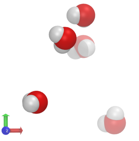
The output, when visualized using VMD, looks like this:

2.2.4. System sizes¶

Let’s start with atoms. The size of an atom is in the scale of Ångströms (10\(^{-10}\) m). Thus, it is quite easy to see that describing anything in macroscopic length scales is simply impossible; just make a simple estimate of how many water molecules would it take to fill a endoscopic container of size 10 nm\(\times\)10 nm\(\times\)10 nm! For reference, if you look at the example .gro file from the dropdown above, the last line gives the dimensions of the simulation box in nanometers: the box length is 1.86206 nanometers. When using the more or less correct density of water, the box can fit a maximum of about 216 water molecules. Since each water has (using the SPC model) three atoms, the total number of atoms is 648.

One advantage of continuum simulations using fields is that it is possible to describe systems in much larger length scales since one is not limited to atoms. What one loses is the atomic specificity and its consequences. There are approaches that allow continuum methods to be more material specific but such a techniques are outside the scope of this course. For those interested, such methods include phase-field[9] and phase-field crystal methods[8].

2.3. Summary¶

This section introduced a number of concepts related particle modeling. In the next sections, we will make these concepts more quantitative and put them into practise when we set up and analyze simulations and simulation data.

2.4. Bibliography¶

1: B. J. Alder and T. E. Wainwright. Phase transition for a hard sphere system. The Journal of Chemical Physics, 27(5):1208, 1957. doi:10.1063/1.1743957.
2: Dominik Fritz, Konstantin Koschke, Vagelis A. Harmandaris, Nico F. A. van der Vegt, and Kurt Kremer. Multiscale modeling of soft matter: scaling of dynamics. Physical Chemistry Chemical Physics, 13(22):10412, 2011. doi:10.1039/c1cp20247b.
3: J. B. Gibson, A. N. Goland, M. Milgram, and G. H. Vineyard. Dynamics of radiation damage. Physical Review, 120(4):1229–1253, nov 1960. doi:10.1103/physrev.120.1229.
4: S. Lifson and A. Warshel. Consistent force field for calculations of conformations, vibrational spectra, and enthalpies of cycloalkane andn-alkane molecules. The Journal of Chemical Physics, 49(11):5116–5129, dec 1968. doi:10.1063/1.1670007.
5(1,2): Siewert J. Marrink and D. Peter Tieleman. Perspective on the Martini model. Chemical Society Reviews, 42(16):6801, 2013. doi:10.1039/c3cs60093a.
2: Nicholas Metropolis, Arianna W. Rosenbluth, Marshall N. Rosenbluth, Augusta H. Teller, and Edward Teller. Equation of state calculations by fast computing machines. The Journal of Chemical Physics, 21(6):1087, 1953. doi:10.1063/1.1699114.
7: Teemu Murtola, Alex Bunker, Ilpo Vattulainen, Markus Deserno, and Mikko Karttunen. Multiscale modeling of emergent materials: biological and soft matter. Physical Chemistry Chemical Physics, 11(12):1869, 2009. doi:10.1039/b818051b.
8: N. Provatas, J. Dantzig, B. Athreya, P. Chan, P. Stefanovic, N. Goldenfeld, and K. Elder. Using the phase-field crystal method in the multi-scale modeling of microstructure evolution. JOM Journal of the Minerals, Metals and Materials Society, 59(7):83–90, July 2007. doi:10.1007/s11837-007-0095-3.
9: Ingo Steinbach. Phase-field models in materials science. Modelling and Simulation in Materials Science and Engineering, 17(7):073001, jul 2009. doi:10.1088/0965-0393/17/7/073001.
10: A. Warshel and M. Karplus. Calculation of ground and excited state potential surfaces of conjugated molecules. i. formulation and parametrization. Journal of the American Chemical Society, 94(16):5612–5625, aug 1972. doi:10.1021/ja00771a014.

CHEM3300G