Lab 3: Simulation of water¶

Learning goals:

To learn how MD simulations work in practise
To learn the basic protocols applied in MD simulations
To understand the difference between energy minimization and simulation
To be able to do the most basic analysis and plot the results
To be able to trace errors and determine how to fix them

Keywords: Particle simulations, molecular dynamics, Monte Carlo, continuum simulations, molecular topology, force field, interactions

Note:

The links are provided for additional information for those interested, not as required reading.
Plotting with xmgrace is the easiest and most straightforward way. You may also plot using Jupyter Lab (that’s how the sample plots were done).

The tasks consist of the following:

Preliminaries: Checking that Gromacs[2] has been installed
Preliminaries: Checking that the systems finds Gromacs
System Setup
Energy minimization
Pre-equilibration
Simulation
Data analysis

All parts involve quick visualizations, error checking and visualizations.

Preliminary: Create yourself a working directory¶

Create a new directory under CHEM3300G. Give the directory a descriptive name. For example, lab_water_1 or something like.
Keep track of the commands and processes. You should have an electronic lab book with notes.

Preliminary: Test that the tools are in place¶

Test if your OS can find Gromacs [5][2]:

which gmx

If yes, then everything is ok.
If not, then you didn’t complete the installation procedure. At the end of installation, the system had to be told where to find Gromacs. Go back to the installation guide and complete the final steps.

Once you have verified that Gromacs (the command gmx) is found by your system, try also the following command:

echo $GMXDATA

If this returns an empty output, then you have not set up Gromacs properly and you should go back to the installation procedure, to part where you have to let the system to know where Gromacs is.

The output should something like this depending where Gromacs is installed:

/home/sam/CHEM3300G/gmx/share/gromacs

If the command worked, you are ready to proceed.

Preliminary: How to get help in Gromacs¶

You can get more information about any command using gmx help <command>. For example, help on Gromacs’ energy calculation:

gmx help energy

The same pattern works for all Gromacs commands. The first part, molecular definitions, is easy since we are simulating water and the model (as well as many other models) already exist and we will be able simply use the model of choice (SPC water [3]).

The other steps have several steps as will be seen.

Important: Always the on-line manual and the help pages if you end up to problems. And if/when you end up to problems, always save the error messages. They tell, or at least give a clue of, what went wrong.

Preliminary: MD workflow¶

The figure below (from lectures) is a reminder of the general MD workflow.

../../_images/molecular-simulation-workflow-simplified.svg

Fig. 2 General MD workflow independent of software. First, one must define the components, that is, the atoms and molecules and their interactions. The atoms and molecules are then used to create the simulation system. After the simulation system has undergone relaxation and pre-equilibration, the actual MD simulation can be started. The simulation produces a trajectory - the coordinates (velocities and forces can be also saved) of all of the particles as a function of time. This trajectory is used for data analysis.¶

Background: Simulation of water using Gromacs¶

Background: Gromacs distribution provides 3 basic water models¶

Gromacs provides 3 basic water models. These models are for

3-point water such as SPC [4], SPC/E [3] and TIP3P [6]
4-point models such as TIP4P [6], TIP4P/2005 [1]
5-point models such as TIP5P [9] and TIP5P/2018 [8]

The corresponding .gro files in the directory $GMXDATA/top and they can be found easily by command

ls -l $GMXDATA/top/*.gro

The output contains lines such as

spc216.gro
tip4p.gro
tip5p.gro

The figure below provides a qualitative explanation of the different models.

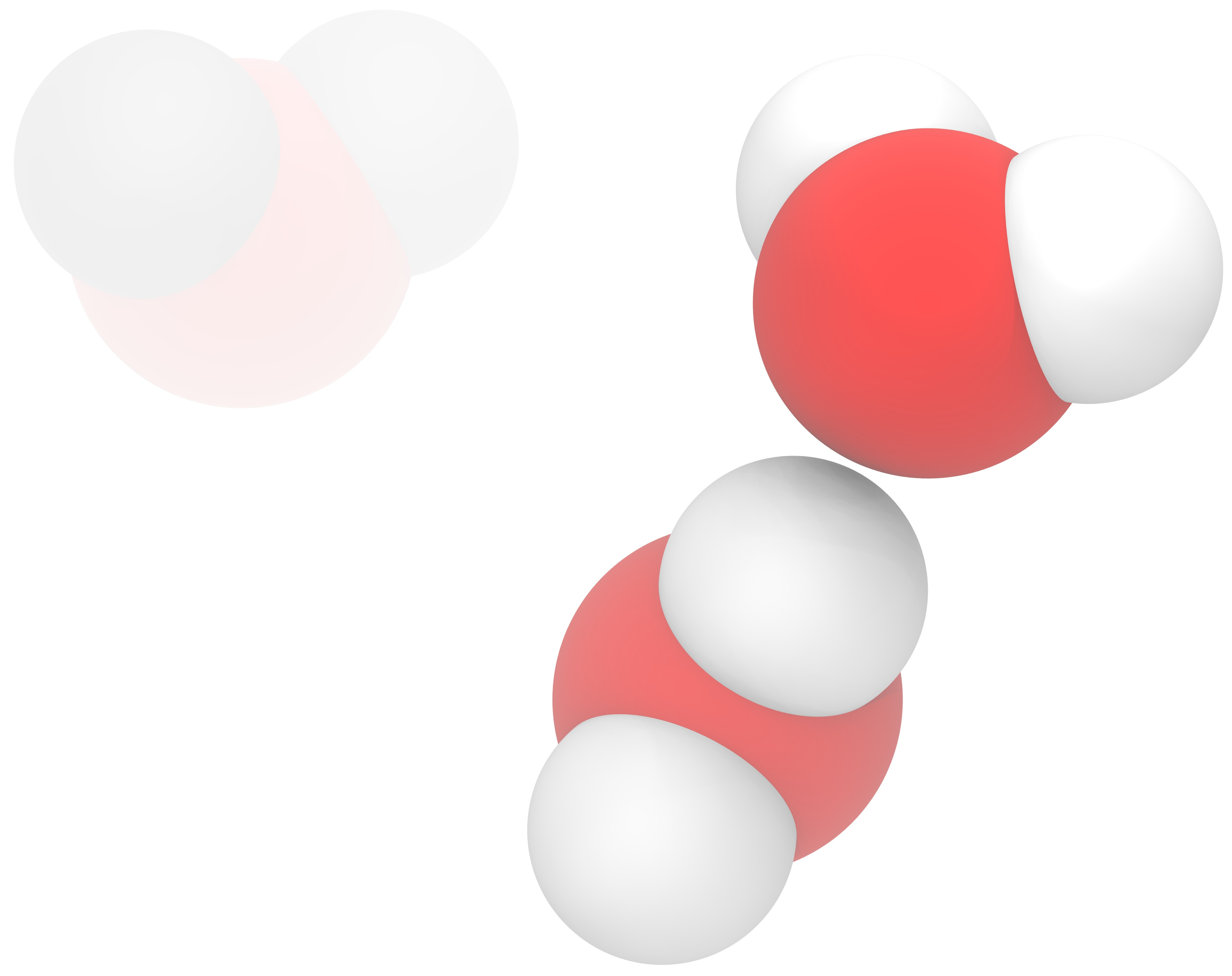
Fig. 3 Different water models Left: A three point model (such as SPC[4] and TIP3P[6]) have three interaction centers. Middle: A four point model (such as TIP4P[6], TIP4P/2005[1]) has four interaction centers. The additional on is a virtual site. Right: A five point model (such as TIP5P[9] and TIP5P/2018[8]) has two virtual sites. Each additional site adds to the computational cost.¶

Background: Notes¶

Gromacs provides several 3-point models: SPC, SPC/E and TIP3P. For all 3-point models the file spc216.gro (located in $GMXDATA/gromacs/top) can be used. There are no separate tip3p.gro or spce.gro and other files. The file spc216.gro contains 216 pre-equilibrated SPC (3-point) molecules.
Gromacs provides one 4-point model (in that same location as the 3-point model), tip4p.gro. The file tip4p.gro has 216 pre-equilibrated (at 300 K) TIP4P water molecules.
Gromacs also provides one 5-point model (again at the same location as the two above): tip5p.gro. Tile tip5p.gro has 512 pre-equilibrated (at 300 K) TIP5P water molecules.
You can, of course, always build your system starting from a single H$_2$O and clone that.
The directory $GMXDATA/gromacs/top has also force field directories, such as
```
gromos54a7.ff
```
within it. Each of these force field directories have their own respective .itp files for the water models to be used with them. In addition, each of these directories has a file
```
 watermodels.dat 
```
which contains some info regarding the force field and the recommended water models. Not all water models can be used with all force fields.

Background: Water models not provided with the Gromacs distribution¶

There are lots of other water models. If you wish use them, you just have to build the topologies, pay attention to force fields and compatibility with possible solutes and their force fields.
Coarse-grained models (such as the Martini model [10]): Must be obtained/built separately.

Background: Notes on setting up the simulation box¶

There are several possible ways to set up a simulation for a water box, we will follow the setup procedure below as it is very general and useful. This is what we will do:

Insert (gmx editconf) the pre-equilibrated 216 water molecules from the spc216.gro centered in a simulation box of chosen geometry (we will use cubic). After setting up the initial system and defining the size (gmx editoconf),
the simulation box is then filled with more water (gmx solvate).

The steps above constitute the system setup process. There are a few things worth repeating before we start:

Use descriptive file names. That is particularly useful if you need to trace back your steps, start new simulations using the same structures, and in finding errors. This is the approach we will follow.
Pay attention to the error messages and other messages the software produces.
Keep also in mind that at almost each step, a new .gro file is created. Using unique and descriptive file names helps to keep track of the .gro files created at various stages.

Background: Homework task¶

What’s the deal with 216 SPC molecule file (spc216.gro) and the box vectors?

Figure it out the answers by finding the solutions to these questions.

Normal density of water is 1 g/cm$^3$
We have 216 water molecules
Mass of a water molecule is: <your answer here>
216 water molecules weigh: <your answer here>
The last line says: <your answer here>
- This gives a box of volume: <your answer here>

Step 1: Generate simulation box¶

Now we can start the procedure. The first step is to generate a simulation box with a desired geometry and choose the boundary conditions (we’ll use periodic boundary conditions or PBC).

See also gmx editconf in Gromacs manual
Note 1: Remember the command source.
Note 2: Below: when necessary, replace username by your own username
Note 3: Unless otherwise said, the commands must be on one single line

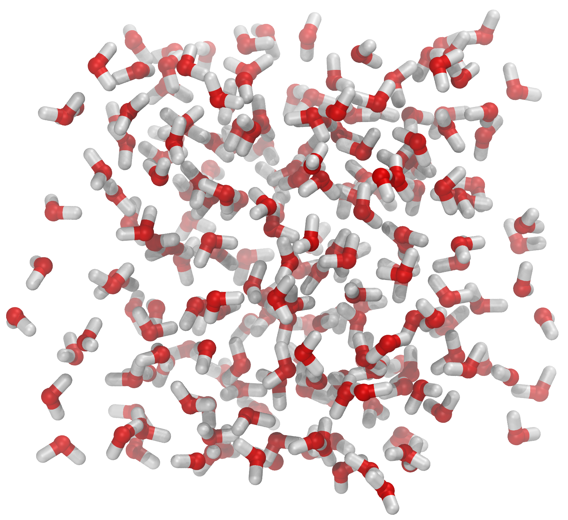
Fig. 4 The file spc216.gro comes with Gromacs[2]. The file contains 216 pre-equilibrated SPC water molecules. You should open the file in VMD and check it yourself. The system has a cubic geometry and the dimensions of the system are given as the very last line of spc216.gro. The dimensions are given in nanometers. One can show the simulation box by opening the Tk shell in VMD and typing pbc box. This is part of the pbctools plugin for VMD and it comes with the basic installation (=you have it).¶

First, we generate a cubic box with side of length 4 nm with the system of 216 waters centered inside it using the command below. Important: this must be on one continuous line so be careful if you are copy-pasting:

gmx editconf -f ${GMXDATA}/top/spc216.gro -o spc216-cubic-4.gro -bt cubic -box 4

Command details:

-f    # input file. Typically .gro, .pdb or .tpr. We use .gro
-o    # output file. Typically .gro
-bt   # box type. 
-box  # Vector length(s) [box size]. For cubic and dodecahedral boxes only one value 
      # is needed. Centers the system (no -c needed). Gromacs uses nanometers.

Step 1: Homework task¶

Pay attention to the output and find the answers to the following questions.

What is the size of the box that was generated?
How do you know that the box is cubic?

Step 1: Notes¶

The box size of 4 nm will give roughly 1,940 water molecules (as you will in the next step). This is ok even with older computers. You can also change it to a smaller number to speed up computations later on, but it should be larger than 2.8. If you change the box size, it may be a good idea to change the name so that it describes what the file contains.

What is happening above: you must have the input file spc216.gro. The 216 water molecules are put inside a new cubic simulation of size 4 nm. You should check both the original spc216.gro and the new file spc216-cubic-4.gro using VMD. The file spc216.gro is the only input file here. A new file is generated as specified by the option -o (stands for output). This new file is called spc216-cubic-4.gro. The number after -box determines the vector length (remember that Gromacs’ units are in nanometers), that is, -box 4 generates a cubic box with a size of 4 nm.

Step 1: What can go wrong¶

Gromacs didn’t find spc216.gro. One possibility is then to copy it from $GMXDATA/top to your current work directory or refer to it directly (that’s what we are doing above).
The above commands must be on a single line so be careful when you copy-paste. The same applies to the rest.

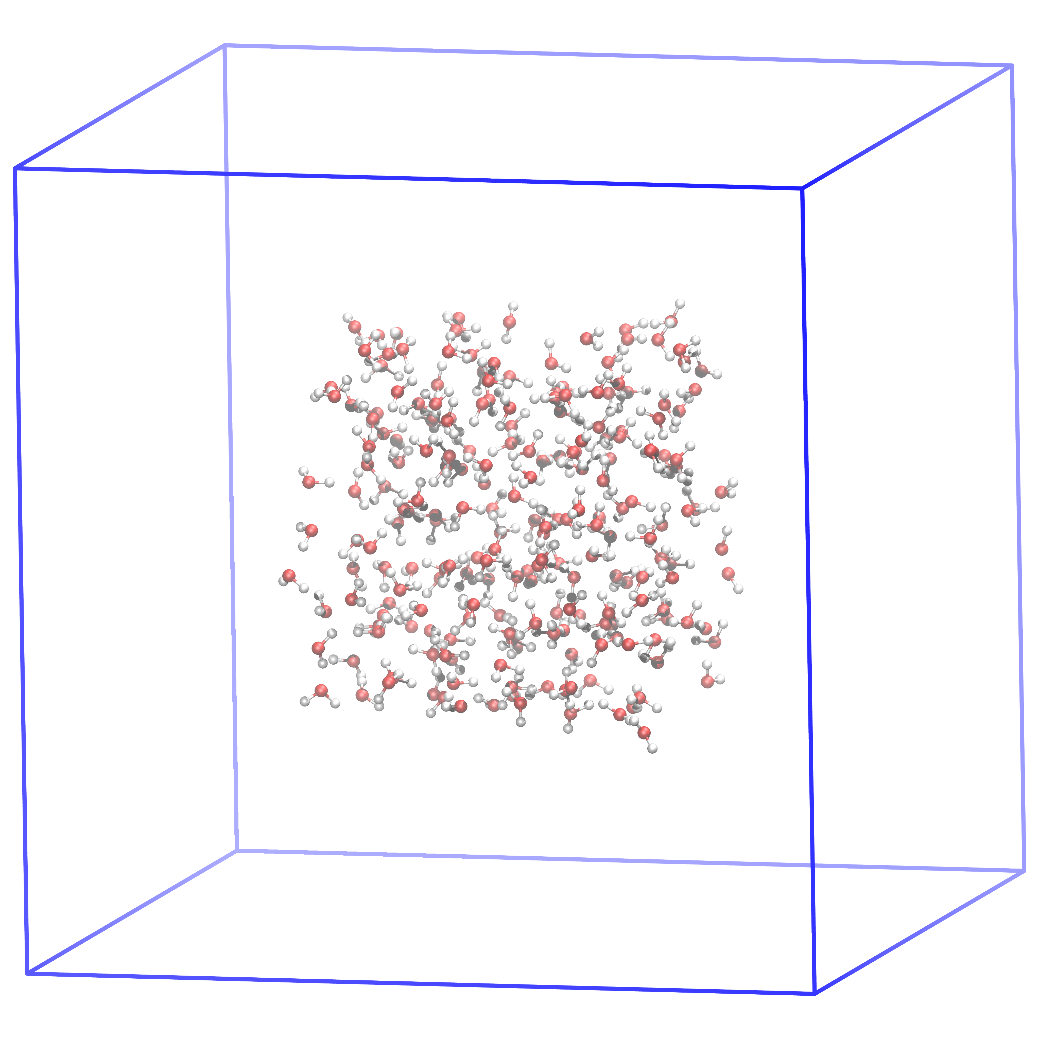
Fig. 5 This is how the system should look like after generating the box and putting the 216 SPC waters in the middle of it. In the next step, we will fill the box with water such that the density is very close to the physical density.¶

Step 2. The simulation box needs to be filled with water.¶

gmx solvate in Gromacs manual

In the previous step, we generated a box of linear size 4 nm and put 216 SPC [3] water molecules in the middle of it. The next command will add more water molecules to fill the box:

gmx solvate -cp spc216-cubic-4.gro -cs spc216.gro -o spc216-solvated-cubic-4.gro

Step 2: Homework task¶

Pay attention to the output and write down (copy-paste) the answer to the following questions. You will need them in the next assignment unless you want to perform this task again.

What is the precise number water molecules?
How many atoms in total?
Were there any overlaps? If so, how many?
What is the exact density of the system?
What are the exact dimensions of the box (hint: you may want to check the new gro file)?

The exact number of molecules will most likely be slightly different for you (and for everyone for that matter). Why? Because the process of solvation involves random numbers. You should check, however, that the density is reasonable.

Command details:

-cp  #	input file. This contains the solute. 
     #  box size is included in this (we defined this with editconf above).
-cs  #	input file. This contains the solvent.
-o 	 #  output file. The part noff just tells that no force field has been incorporated yet. 

After completing Step 2, we have the initial structures ready. We have not, however, associated force fields with them or any other parameters for that matter – if you have used Gromacs[2] before to, say, solvate a protein, you notice that we did not specify a topology file above. This is what we will do next.

You should open the file spc216-solvated-cubic-4.gro in VMD and see how the system looks like.

Although the small 216 water molecule system was equilibrated, these larger new systems are not. We used the small 216 molecule system since it was pre-equilibrated with a density close to real water density. By multiplying that system, we obtained a new larger one that has density close to what the density of water should be. The new system is, however, not in equilibrium.

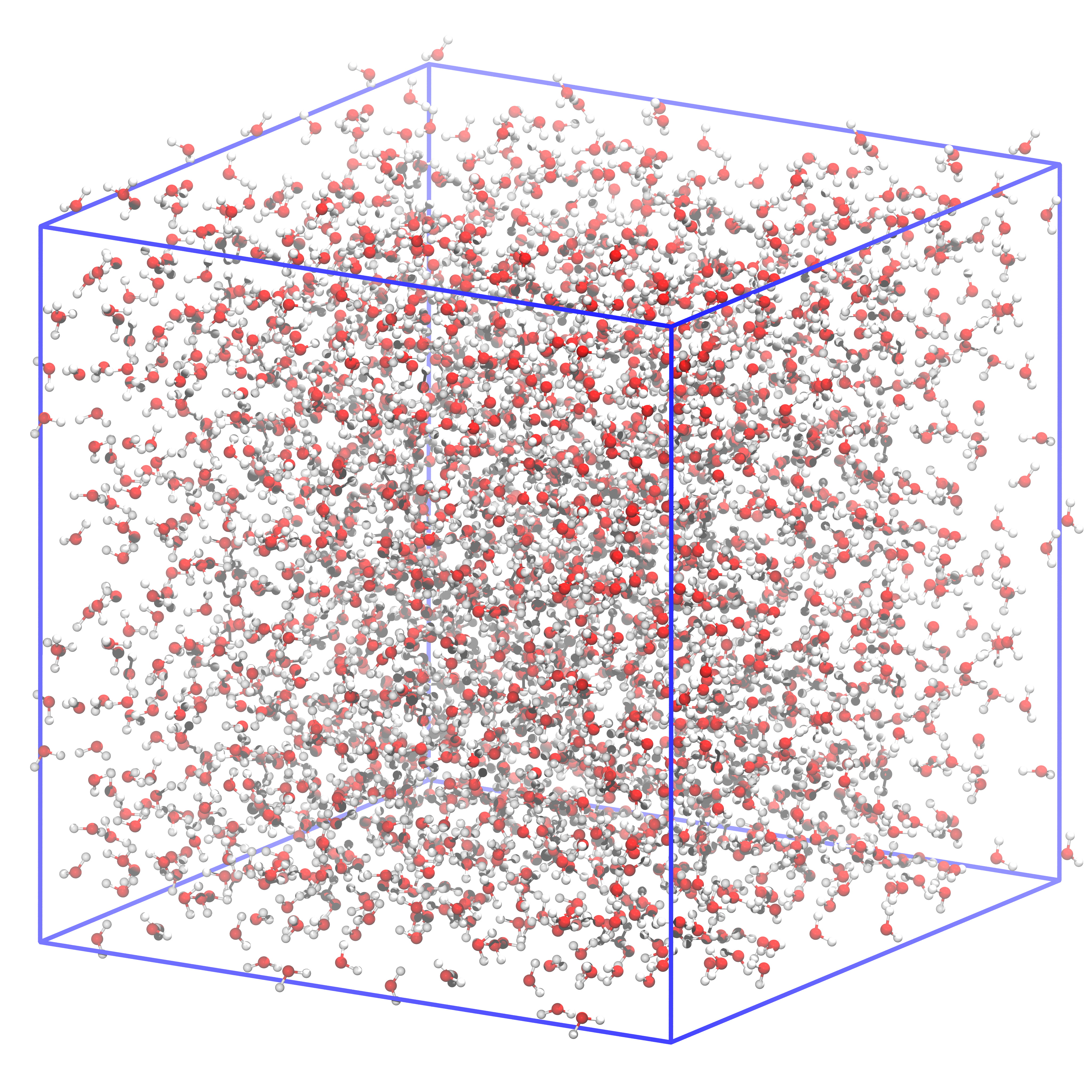
Fig. 6 This is how the system filled with water should look like. The box size is precisely the same as in the previous figure.¶

Step 3. Generate the topology and index files¶

The above procedure defined the initial coordinates but not the force fields and topologies. This is done with the command gmx pdb2gmx.

When executed, pdb2gmx

asks for a force field and the specific water model

So far we have only defined the water model to be a 3-site model instead of 4- or 5-site model but we have not defined if the model is SPC [3], SPC/E [3] or TIP3P [6]. These models are all 3-site models and we have to choose one of them. In our case, we will choose SPC (but could have equally well chosen one of the others).

Topology: defines the molecular connections. In Gromacs [2], there are three types of topology files: 1) .itp for individual molecules. The file gives the connectivity information for the different atoms, atomic charges, angles and so on. 2) The files having the suffix .top are system topology files. They contain topology description for the simulation system. 3) The final one is residue topology. These files have the suffix .rtp. They are for proteins and are used by the Gromacs routine pdbgmx.

Here, we use .itp files implicitly (they are already included in the force field description and we don’t have to do anything about them). We generate a system topology (.top) file. Since we don’t have any proteins, .rtp files are not used here.

Note: The command gmx pdb2gmx below produces 3 files: topology, position restraints and .gro (or other specified).

Generate a cubic simulation box:

gmx pdb2gmx -f spc216-solvated-cubic-4.gro -o spc-oplsaa-solvated-cubic.gro -p spc-oplsaa-solvated-cubic.top -n spc-oplsaa-solvated-cubic.ndx

When prompted, select OPLS-AA (Optimized Parameters for Liquid Simulations) [7] for the force field and SPC (Simple Point Charge) [4] for the water model. The output files above have been named with that assumption. Change the names if you change the force field / water model.

Pay attention to the messages if there are any errors or warnings.

Again, select OPLS-AA [7] for the force field and SPC [4] for the water model.

Command details:

-f 	 # input file. 
-o 	 # output file.
-p 	 # output file. Topology.
-n 	 # output file. Contains reordered groups.

The dropdowns below show sample outputs during the process.

Step 3: Homework task¶

The title mentions index file. Find the Gromacs manual from the web and explain in your own words hat an index file is and for what it is needed.

Step 4. Run the grompp pre-processor.¶

This generates the run file for relaxation

gmx grompp in Gromacs manual

This is the first time we use grompp and we do need a .mdp file. The suffix mdp comes from Molecular Dynamics Parameters. As the name suggests, that file contains the various parameters for the simulation.

This .mdp file must be created before executing the commands below. The .mdp file contains all the runtime parameters and protocols. However, for the minimization step, very little is needed.

To do: The .mdp file for energy minimization can be as simple as the one below in the dropdown. It must be plain ASCII. Generate this file now – otherwise the command below will not work. Name the file em.mdp:

This is an energy minimization step (not a true simulation) and since we are using deterministic optimization, some of the above parameters are not critical. It is, however, good to set the correctly from the beginning (pme, etc.).

Why do we need to do this? Inserting molecules in the system is more or less a random process. There may be steric problems (=partial overlaps or too much empty space between the molecules). Conformations may be energetically very unfavourable and so on. Thus, the structure needs to be relaxed. It is important to keep in mind that energy minimization is not an actual simulations. It is simply a process in which the energy is minimized based on the positions of the molecules, time is not involved and Newton’s equations of motion are not solved. The two most common minimization methods are the method of steepest descents and the conjugate gradient method. We will not go into detail here, but they are so-called deterministic optimization methods.

Notice: The same .mdp file is good for both of the cubic and dodecahedral cases (as well as others).
Important: The grommp command below combines information from em.mdp and the solvated system we created above and generates a run input file (.tpr)
Notice: When you execute the commands below, pay attention to possible errors / warnings.

gmx grompp -v -f em.mdp -c spc-oplsaa-solvated-cubic.gro -p spc-oplsaa-solvated-cubic.top -o spc-oplsaa-solvated-cubic-minimize

This generates a run input file named spc-oplsaa-solvated-cubic-minimize.tpr. The suffix .tpr denotes a run input file and as the name suggests, that file is used for running a simulation or a minimization procedure. The latter will be done in the next step using this file.

Command details:

-v 	# verbose mode. Show all the messages. 
-f 	# input: the .mdp file.
-c 	# input file. Structure as generated above.
-o 	# output file. The run input file of .tpr type.

Output from grompp for energy minimization

GROMACS:      gmx grompp, version 2020.4
Executable:   /data/TEACHING/CHEM3300G/gmx/bin/gmx
Data prefix:  /data/TEACHING/CHEM3300G/gmx
Working dir:  /data/TEACHING/CHEM3300G/water_1/Lab
Command line:
  gmx grompp -v -f em.mdp -c spc-oplsaa-solvated-cubic.gro -p spc-oplsaa-solvated-cubic.top -o spc-oplsaa-solvated-cubic-minimize

checking input for internal consistency...

NOTE 1 [file em.mdp]:
  With Verlet lists the optimal nstlist is >= 10, with GPUs >= 20. Note
  that with the Verlet scheme, nstlist has no effect on the accuracy of
  your simulation.

Setting the LD random seed to -1426617453
processing topology...
Generated 330891 of the 330891 non-bonded parameter combinations
Generating 1-4 interactions: fudge = 0.5
Generated 330891 of the 330891 1-4 parameter combinations
Excluding 2 bonded neighbours molecule type 'SOL'
processing coordinates...
double-checking input for internal consistency...
renumbering atomtypes...
converting bonded parameters...
initialising group options...
processing index file...
Analysing residue names:
There are:  2162      Water residues
Making dummy/rest group for T-Coupling containing 6486 elements
Making dummy/rest group for Acceleration containing 6486 elements
Making dummy/rest group for Freeze containing 6486 elements
Making dummy/rest group for Energy Mon. containing 6486 elements
Making dummy/rest group for VCM containing 6486 elements
Number of degrees of freedom in T-Coupling group rest is 12969.00
Making dummy/rest group for User1 containing 6486 elements
Making dummy/rest group for User2 containing 6486 elements
Making dummy/rest group for Compressed X containing 6486 elements
Making dummy/rest group for Or. Res. Fit containing 6486 elements
Making dummy/rest group for QMMM containing 6486 elements
T-Coupling       has 1 element(s): rest
Energy Mon.      has 1 element(s): rest
Acceleration     has 1 element(s): rest
Freeze           has 1 element(s): rest
User1            has 1 element(s): rest
User2            has 1 element(s): rest
VCM              has 1 element(s): rest
Compressed X     has 1 element(s): rest
Or. Res. Fit     has 1 element(s): rest
QMMM             has 1 element(s): rest
Calculating fourier grid dimensions for X Y Z
Using a fourier grid of 36x36x36, spacing 0.111 0.111 0.111
Estimate for the relative computational load of the PME mesh part: 0.26
This run will generate roughly 1 Mb of data
writing run input file...

There was 1 note

GROMACS reminds you: "Don't Follow Me Home" (Throwing Muses)

Step 4: What can go wrong¶

This should be a straightforward step: Information is just collected into the run input file (.tpr) to be used in the next step.

Step 4: Homework task¶

Go to the Gromacs manual and read what the parameters integrator, nsteps and pbc are. Explain (in your own words) their significance.

Step 5: Relaxation using energy minimization (steepest descents or conjugate gradient)¶

gmx mdrun in Gromacs manual

Now that we have our run input files (.tpr), we can perform energy minimization, that is, to relax the systems. This process is there to ensure that possible steric conflicts will be take care of. In other words: it may have happened that during solvation some of the molecules were put in too close contact or too far way from each other. The former leads to enormous energies (atoms cannot overlap) and the latter can lead to the molecules accelerating too fast when the actual simulation starts.

We have now defined the initial structures, topologies and force field. In this step we apply the method of steepest descents (conjugate gradient would work as well) to relax the system. Notice that both steepest descents and conjugate gradient are methods of deterministic optimization, they are not real simulations (that sounds like an oxymoron…). In other words, the process will stop when they the first local energy minimum is found. This means that 1) it is sometimes a good idea to repeat this after the Equilibration (next) and 2) increasing the number of relaxation steps does not lead to better convergence since these algorithms stop after they find the first local minimum.

Important: If you for some reason wish to change the parameters in the .mdp file at this time, you must return to previous stage and re-run it.

We use cubic geometry:

gmx mdrun -v -deffnm spc-oplsaa-solvated-cubic-minimize

The syntax:

mdrun       # obvious
-v          # verbose output so that you can follow what is happening
-deffnm	    # file names for input and output (all files will be named using this)

The following files will be generated by mdrun:

[filename].log		# log file
[filename].edr		# energy. Binary file
[filename].trr		# Trajectory. Full precision, binary format.
[filename].gro		# Energy minimized structure

where [filename] is either water-cubic-minimize or water-dode-minimize.

Check that energy converged

gmx energy -f spc-oplsaa-solvated-cubic-minimize -o energy-check.xvg

This gives you a menu you can use to select which quantities(s) you want to plot. The very least you should look at the potential energy. You can view the .xvg file with xmgrace (if you use Matlab or something else, you may need to change the comment style in the file; if you do so, you must again use an ASCII editor).

If everything looks more or less ok, you can proceed to the next step (=the problem was not a serious one). In the not so fortunate case, you have two choices: 1) try to produce a new file starting from the beginning or 2) use one of the .pdb files produced during minimization, identify the problematic molecule and rotate or move it slightly and try again (by editing the file, using VMD or other software).

Fig. 7 Potential energy as a function of minimization steps taken. Notice that if you print the generated file directly using xmgrace, the label of the x-axis is wrong and you should correct it. In this case, there was no full convergence before the maximum number of steps (1000) was reached. However, inspection of error messages, plotting the energy and inspecting the files indicated in the error messages shows that there was no real problem.¶

Step 5: Homework task:¶

Answer the following questions using your own results:

How many picoseconds did it take for the minimization to converge?
How do you know if the minimization actually worked out?
What other possible methods there are for energy minimization (=methods)?
Use VMD to visualize how the minimization process worked: pick residues 10 and 11, and superimpose the the starting structure and the minimized structure. Color the molecules In the initial structure in red and in the optimized structure in orange.
Based on the previous question: Describe the rotations and translations of the two water molecules (residues 10 and 11). Explain your observations.

Step 6: Pre-equilibration run in the NVE ensemble¶

In this step, we will perform an NVE (constant particle number, volume and energy) simulation – this is a real MD simulation unlike the minimization step above (the minimization is technically speaking deterministic optimization).

In this simulation, we keep the number particles (N), volume (V) and energy (E) constant. To be able to do all that, a new .mdp file is needed, the previous one cannot be used. You must create a new file (the one below) and I suggest you name it nve-equib.mdp. Remember that it must be an ASCII file, this is an absolute requirement. Notice also how there are comments in the .mdp file. Always put in comments, they are very helpful.

nve-equib.mdp

;=================================================================
; Fairly minimal mdp file for NVE equilibration
; Name: nve-equib.mdp
; If in doubt: http://manual.gromacs.org/online/mdp_opt.html
;==================================================================
;
;  No position restraints in this one. If needed, add them here.
;
;== RUN CONTROL. Time in ps.  =================================
;
title		= NVE equilibration of SPC water
integrator 	= md 		; standard leap-frog. others are available incl. vv
dt		    = 0.001		; time step in ps. No constraints: 0.001, w/: 0.002.
nsteps		= 20000 	; # of steps. This would mean 20 ps for MD (20000*0.001). 
comm-mode	= linear	; removes both translation and rotation of COM (center of mass).
nstcomm		= 100		; frequency (in steps) to remove COM motion
;
;== NEIGHBOR LISTS ============================
;
cutoff-scheme 	= Verlet	; Verlet is needed for GPU. Works with CPUs too
nstlist 	    = 20		; neighbor list update frq. Verlet: 20-40, group <10. 20 fs.
ns_type		    = simple	; method for constructing neighbor lists. Grid is faster
pbc		        = xyz		; Full periodic boundary conditions
verlet-buffer-tolerance = 0.005 ; May have to use smaller value for NVE but let’s start with this
;
;== OUTPUT CONTROL ===================================================
;
nstxout		= 500		; write out coordinates every 0.5 ps. Standard: 1.0 ps
nstvout		= 500		; frq for writing out velocities
nstenergy	= 500		; frq for writing out energies
nstlog		= 1000		; frq for updating the log file
; 
;== Electrostatics. Default order: 4, tol: 1e-5, spacing: 0.12 nm, geom: 3d ==
;
coulombtype	= pme		; you really do want to use PME instead of cutoff
rcoulomb	= 1.0		; Coulomb real space cutoff
;
;== Van der Waals interactions.================================
;
; rvdw MUST be chosen to be commensurate with rcoulomb
;
vdwtype		= cut-off	; 
rvdw		= 1.0		; vdW cutoff. 
dispcorr	= EnerPres	; Dispersion correction applied to energy & pressure
;
;== TEMPERATURE COUPLING: NVT / NpT RUNS=======================
;
tcoupl		= no		; NVE RUN needs no thermostat
;
;== PRESSURE COUPLING: NpT RUNS =====================
;
pcoupl		= no		; NVE RUN (use this also for NVT) needs no barostat
;
;== GENERATE VELOCITIES: NEEDED FOR EQUILIBRATION AND SET UP =======================
;
; NOTE: gen_vel = no if the run is a continuation! 
;
gen_vel		= yes		; generate velocities from a Maxwell distribution
gen-seed	= -1		; random seed for random number generation 
gen_temp	= 300		; temperature for the above Maxwell distribution
;
;== Continuing a previous simulation? ======================================
;
; Also needed when running back-to-back equilibration runs! (NVT-> NpT)
; IMPORTANT: You may need to set gen_vel=no above. 
; 
continuation	= no 		; restarting a previous run?
;
;====================================================================================

Now that you have nve-equib.mdp generated, we must grompp again. As above, grompp takes the parameter file (nve-equib.mdp), the file after minimization and created a run input file.

Step 6.1: Grompp to set up an NVE run¶

In the previous step we minimized energy. The reason for that was to remove possible unphysical voids or/and molecular overlaps. The next step is to run a short simulation to ensure that the system is stable. If not, we need to go back to the setup procedure and solve possible problems. The first simulation is done in the NVE ensemble. For that we need a new .mdp file with some new parameters. We also need to generate a new run input - the previous one was for minimization only.

The above means that we need to run the grompp preprocessor and use the new .mdp file. This process again combines the input parameters (nve-equib.mdp), topology and the minimized structure from the last step:

gmx grompp -f nve-equib.mdp -c spc-oplsaa-solvated-cubic-minimize.gro -p spc-oplsaa-solvated-cubic.top -o spc-oplsaa-cubic-nve.tpr

Pay close attention to the messages grompp produces. This process produces a new run input file (.tpr). It will be needed in the next step for the NVE simulation.

-f nvt.mdp	  ; input, not modified. Uses posres.top
-c em.gro	  ; the structure for energy minimization as input. not modified
-p topol.top  ; topology
-o nvt.tpr	  ; trajectory. Output. Modified	

Step 6.2: Perform pre-equilibration NVE run.¶

Now we are ready to simulate. The following command runs a short (20 ps) real NVE molecular dynamics simulation:

gmx mdrun -s spc-oplsaa-cubic-nve.tpr -o -x -deffnm spc-oplsaa-cubic-nve-run

Note: This leaves the command running on the foreground. Completion shouldn’t take too long:

On an i7 laptop with NVIDIA GTX1070 this took 4.9 seconds (CUDA 11.0, gcc 9.3.0)
One an -7 laptop with 12 cores it took about 20 seconds
Shouldn’t take more than 2 minutes even on an old computer. You can put it in the background by adding & character to the end of the line. There are also other ways of doing that but we will discuss them later.
As a separate benchmark: On an i7 laptop with NVIDIA GTX1070 running 1 ns took 268 seconds (CUDA 11.0, gcc 9.3.0)

Command details:

mdrun 	  # obvious
-s 		  # run input file. Typically .tpr (the one created in the above step)
-x 		  # produces compressed trajectory (xtc)
-o 		  # produces full precision trajectory
-deffnm	  # file names (all files will be named using this)

At the end, you will get the details of the execution time and other stuff. Pay attention to the messages. Here is a sample:

starting mdrun '216H2O,WATJP01,SPC216,SPC-MODEL,300K,BOX(M)=1.86206NM,WFVG,MAR. 1984'
20000 steps,     20.0 ps.

Writing final coordinates.

               Core t (s)   Wall t (s)        (%)
       Time:      206.962       17.247     1200.0
                 (ns/day)    (hour/ns)
Performance:      100.197        0.240

Again, you should take a look at what is going on using VMD.

You can even seen an on-screen movie: first load the .gro file (spc-oplsaa-cubic-nve-run.gro) in VMD and then use the “Load data into molecule” option in VMD to load the .trr file (spc-oplsaa-cubic-nve-run.trr is, the trajectory; the trajectory contains the coordinates at different times as defined by the parameter nstxout in the .mdp file).

You should also take a look at the different quantities. The first one to take a look at is total energy since in an NVE simulation the total energy must be conserved. It is also interesting to take a look at kinetic energy and potential energy.

We use the same procedure as above:

gmx energy -f spc-oplsaa-cubic-nve-run -o energy-check-nve.xvg

As above, create plots of the data and interpret what they indicate.

Here are sample plots, yours will be, obviously, somewhat different.

Step 6: Homework task¶

Answer the following questions using the plots below:

Examine the 3 different energies. Is the system well-behaved or are there indications of problems? Provide clear reasons for your answer.
Kinetic energy increases. What was the starting temperature? What is the final temperature (approximately)? How large is the increase?
Why does kinetic energy increase and potential energy decrease?
What can be done to maintain constant temperature?
NVE ensemble is, by definition, constant energy. Discuss the behavior of the total energy.
Compare your plots to these. Are there differences? Describe them and justify their origin.

../../_images/energy_check-nve-kinetic.svg

Fig. 8 The figure shows kinetic energy as a function of time. It doesn’t appear to be constant. What does that indicate? Is this a problem?¶

../../_images/energy_check-nve-potential.svg

Fig. 9 Potential energy as a function of time. After initial decrease, the value seems to settle. Why is that?¶

../../_images/energy_check-nve-total.svg

Fig. 10 Total energy as a function of time. This is a result from a constant energy (NVE) simulation. The energy doesn’t seem constant. Does that indicate a problem? In addition, pay attention to the data point at time equals to zero.¶

Step 7: Set up a pre-equilibration NVT run¶

After the brief NVE run, let’s perform an NVT (constant particle number, volume and temperature; this is the canonical ensemble – NVE is called the microcanonical ensemble) run. For this, the .mdp file needs modifications in the respective sections as given below. Let’s save a copy of the current NVE .mdp file under the name nvt-equilib.mdp and make the changes in this new file. Then make the changes as indicated below. As you see, some new parameters come into play.

Makes these changes to the .mdp file and

tcoupl       = v-rescale  ; NVT RUN
ref_t        = 300		  ; temperature in Kelvin
tau_t        = 0.1		  ; time constant for coupling. 0.1 ps
tc_grps	     = System	  ; Let's put the whole system on single thermostat
gen_vel	     = no		  ; we continue our previous run
continuation = yes 		  ; restarting a previous run
gen_vel	     = no		  ; we continue our previous run
continuation = yes 		  ; restarting a previous run

Important: If you took a look at the directory in which you performed the NVE run, you noticed that there is also a new file, a .cpt file. That is a checkpoint file (binary) and it will be used when restarting. There is also a .gro file that was written at the same time. That contains the coordinates from the final stage of the simulations and they will be used for the restart.

Below is the grompp command. Notice that the topology file is still the same. Makes sense since the molecular connectivity has not changed.

gmx grompp -f nvt-equib.mdp -c spc-oplsaa-cubic-nve-run.gro -t spc-oplsaa-cubic-nve-run.cpt -p spc-oplsaa-solvated-cubic.top -o spc-oplsaa-cubic-nvt.tpr

Command details:

-f          ; input, not modified. Uses posres.top
-c          ; the structure from energy minimization. not modified
-p          ; topology
-o          ; trajectory. Output. Modified	
-t          ; continuation for a previous run (.cpt file) 

Step 7.1: Start the NVT equilibration run¶

We can now run an NVT simulation. Since we are continuing the previous simulation using the .cpt it generated, we just continue where we left off after NVE. Whether or not that is necessary depends on the situation.

gmx mdrun -s spc-oplsaa-cubic-nvt.tpr -o -x -deffnm spc-oplsaa-cubic-nvt-run

Command details:

mdrun     # obvious
-s        # run input file. Typically .tpr (the one created in the above step)
-x        # produces compressed trajectory (xtc)
-o        # produces full precision trajectory
-deffnm   # file names for input and output (all files will be named using this)

Here are the benchmarks, the run took just over 17 seconds:

               Core t (s)   Wall t (s)        (%)
       Time:      209.866       17.489     1200.0
                 (ns/day)    (hour/ns)
Performance:       98.810        0.243

As above, perform the simple energy analysis using

gmx energy -f spc-oplsaa-cubic-nvt-run -o energy-check-nvt.xvg

and create plots of the data and interpret what the plots indicate.

Step 7: Homework Task¶

Answer the following questions using the plots below and your own results:

The first data point in the plots is from the final point of the previous NVE simulation. It seems that for all of the energy components, there is a very large jump. Is that indicative of a problem? Explain your answer carefully.
The kinetic energy seems to settle around 16,000 kJ/mol. Is that correct, too large or too small? Calculate the temperature to what 16,000 kJ/mol corresponds for this particular system.
Compare the kinetic energy to your simulation. Is it the same? Calculate the temperature for your simulation.
This is an NVT simulation, that is constant temperature. Kinetic energy and temperature are related. It seems that the kinetic energy is not constant. Is that a problem? Explain carefully.

Sample plots:

../../_images/energy_check-nvt-kinetic.svg

Fig. 11 Kinetic energy as a function of time. Time 20 ps is the starting point for the NVT simulation after the initial NVE one. Kinetic energy appears to make a quick jump at the beginning and then fluctuate around a constant value. This is a constant temperature simulation: Are such fluctuations indicative of an error or an underlying problem?¶

../../_images/energy_check-nvt-potential.svg

Fig. 12 Potential energy as a function of time. Time 20 ps is the starting point for the NVT simulation after the initial NVE one. The behavior is very similar to what kinetic energy shows. Potential energy seems to increase. Is this behavior reasonable?¶

../../_images/energy_check-nvt-total.svg

Fig. 13 Total energy. energy as a function of time. Time 20 ps is the starting point for the NVT simulation after the initial NVE one. Why does the total energy increase rapidly at the beginning. The total energy is, of course, the sum of potential and kinetic energies. But why doesn’t it stay constant?¶

Step 8: Final simulation in the NpT ensemble¶

So far we have performed short simulation runs in the NVE and NVT ensembles. Now we will perform an NpT (constant particle number, pressure and temperature; this is also the canonical ensemble) simulation. We start the simulation starting from where we left off after the NVT run.

First we need, however, to grommp again. This also means that the .mdp file needs to be modified again since NpT has its own requirements. Remember: the letter p means constant pressure. This allows the simulation box to adjust to the pressure (and hence density will fluctuate). That means we have to let the system size to change and for that we have to have a barostat (Parrinello-Rahman below).

Below are the changes to the .mdp file, copy the previous file to create a new called npt-equilib.mdp and make the changes as indicated below in that:

pcoupl           = parrinello-rahman	; sets a parrinello-rahman barostat
pcoupltype       = isotropic		    ; isotropic coupling
tau_p            = 2.0			        ; coupling time, 2 ps
ref_p            = 1.0			        ; pressure in bars
refcoord-scaling = all			        ; all coordinates scaled
compressibility	 = 4.5e-5		        ; as it says, compressibility

Now we must grompp.

gmx grompp -f npt-equib.mdp -c spc-oplsaa-cubic-nvt-run.gro -t spc-oplsaa-cubic-nvt-run.cpt -p spc-oplsaa-solvated-cubic.top -o spc-oplsaa-cubic-npt.tpr

Step 8.1: Run an NpT simulation.¶

After all that grompping, we are now ready to run an NpT simulation:

gmx mdrun -s spc-oplsaa-cubic-npt.tpr -o -x -deffnm spc-oplsaa-cubic-npt-run

Command details:

mdrun       # obvious
-deffnm	    # file names for input and output (all files will be named using this)

Step 8: Homework task¶

Answer the following questions using your own results:

This is an NpT simulation, that is constant temperature and pressure. Plot 1) pressure and 2) the dimensions of the simulation box. In the case of the dimensions, you should plot x, y and z-dimensions in the same graph.
Are temperature and pressure constant (you need plots)? Explain your observations very carefully.
Discuss why and when one would use NVE, NVT and NpT simulations. Discuss the following: Should one expect the same results from all of them? In particular: If we would perform long simulations of the water system using NVE, NVT and NpT, should we expect the same results in terms of thermodynamic properties, hydrogen bonding, coordination and such?
You have now ran 20 ps simulations using NVE, NVT and NpT ensembles. Is 20 ps long or short? More importantly, is it enough? How can one determine the appropriate length of a simulation. Discuss and justify your answers carefully.
Use VMD to make a movie of the system.

Kinetic energy and temperature are related. It seems that the kinetic energy is not constant. Is that a problem? Explain carefully.

References¶

1(1,2): J. L. F. Abascal and C. Vega. A general purpose model for the condensed phases of water: tip4p/2005. The Journal of Chemical Physics, 123(23):234505, 2005. doi:10.1063/1.2121687.
2(1,2,3,4,5): Mark James Abraham, Teemu Murtola, Roland Schulz, Szilárd Páll, Jeremy C. Smith, Berk Hess, and Erik Lindahl. GROMACS: high performance molecular simulations through multi-level parallelism from laptops to supercomputers. SoftwareX, 1-2:19–25, sep 2015. doi:10.1016/j.softx.2015.06.001.
3(1,2,3,4,5): H. J. C. Berendsen, J. R. Grigera, and T. P. Straatsma. The missing term in effective pair potentials. The Journal of Physical Chemistry, 91(24):6269–6271, Nov 1987. doi:10.1021/j100308a038.
4(1,2,3,4): H. J. C. Berendsen, J. P. M. Postma, W. F. van Gunsteren, and J. Hermans. Interaction models for water in relation to protein hydration. In The Jerusalem Symposia on Quantum Chemistry and Biochemistry, pages 331–342. Springer Netherlands, 1981. doi:10.1007/978-94-015-7658-1_21.
5: Berk Hess, Carsten Kutzner, David van der Spoel, and Erik Lindahl. GROMACS 4: algorithms for highly efficient, load-balanced, and scalable molecular simulation. Journal of Chemical Theory and Computation, 4(3):435–447, Mar 2008. doi:10.1021/ct700301q.
6(1,2,3,4,5): William L. Jorgensen, Jayaraman Chandrasekhar, Jeffry D. Madura, Roger W. Impey, and Michael L. Klein. Comparison of simple potential functions for simulating liquid water. The Journal of Chemical Physics, 79(2):926–935, jul 1983. doi:10.1063/1.445869.
7(1,2): William L. Jorgensen and Julian Tirado-Rives. The OPLS [optimized potentials for liquid simulations] potential functions for proteins, energy minimizations for crystals of cyclic peptides and crambin. Journal of the American Chemical Society, 110(6):1657–1666, mar 1988. doi:10.1021/ja00214a001.
8(1,2): Yuriy Khalak, Björn Baumeier, and Mikko Karttunen. Improved general-purpose five-point model for water: TIP5p/2018. The Journal of Chemical Physics, 149(22):224507, dec 2018. doi:10.1063/1.5070137.
9(1,2): Michael W. Mahoney and William L. Jorgensen. A five-site model for liquid water and the reproduction of the density anomaly by rigid, nonpolarizable potential functions. The Journal of Chemical Physics, 112(20):8910, 2000. doi:10.1063/1.481505.
10: Siewert J. Marrink, H. Jelger Risselada, Serge Yefimov, D. Peter Tieleman, and Alex H. de Vries. The MARTINI force field: coarse grained model for biomolecular simulations. The Journal of Physical Chemistry B, 111(27):7812–7824, jul 2007. doi:10.1021/jp071097f.