Brief introduction to Python#

Learning goals:
- To learn the basics of python.
- To learn how to use Jupyter Lab/Notebook.
Keywords: Python, Jupyter Notebook, Jupyter Lab
Associated material:
- Introduction to Jupyter with screenshots and explanations of the interface
On the web:

Important

Important note: Python 2 has been phased out. The last release was python 2.7.18 on April 20, 2020. The latest release (Nov. 2020) is python 3.9). The codes in this section have been tested with python 3.8.

Python, what is it good for?#

War, what is it good for? Absolutely nothing! Ho!”

—Elaine Benes in Seinfeld

Since its introduction in 1998, Python has become one of the world’s most popular programming languages and often required for jobs that involve any programming.

Python is a modern interpreted language, as opposed to compiled programming languages such as C, C++, Fortran, Pascal, and so on. Being an interpreted language means that the Python interpreter reads the code line-by-line as it is executed. In contrast, a compiled language has to be run through a compiler to produce an executable program. The compiled executable works only on the platform where it was compiled, but a code that is interpreted is more portable between different platforms.

Python was originally created by Guido van Rossum, a Dutch programmer. The first Python implementation was done in December 1989 by van Rossum – to keep himself busy, as he says. Current version of Python is 3 and, importantly, Python 2 has been deprecated and won’t be maintained after 2020.

Below, some properties of Python are listed.

Properties:

General purpose and Jupyter provides interactivity, free and open source.
Dynamically typed (as opposed to statically typed). This means that one doesn’t have to declare variables.
Object oriented.
Portable (Linux, Unix, OSX, Windows, mobile phones…).
Versatile. Python is used in an enormous number of different applications, commercially, in research and in industry.
Easy to learn. This is indeed the case! The barrier to start using Python is very low.
Extensible, it uses modules. The number of available modules is very large.

Disadvantages:

Speed can be an issue since Python is an interpreted language. However, there are efficient libraries and the possibility to use tools such as Cython and even GPUs.

Famous examples/applications/users:

YouTube, reddit, Yahoo, Google (Gmail, Groups, Maps), CERN, NASA.
Part of the core components in Linux distributions.
Information security industry.
Applications such as Abaqus, Gimp, Inkscape, Spotify…

Huge number of modules and libraries. Examples:

SciPy, Biopython, NumPy, Matplotlib, Sage, Tensorflow, Chempy, MDAnalysis, pyEMMA, RDKit, nglview, DeepChem

Used as a scripting language in:

Blender, Gimp, Inkscape, Totem, SPSS, PyMOL

Other:

Jython: compiler that produces Java byte code from a python code
PyS60: Symbian [obsolete now] phones
Python for Android

It is hard to tell exactly how popular Python is (since it is not easy to define a good metric), but in both StackExchange and Github it ranks among the most popular ones. When it comes to programming and programming languages, it is good to keep in mind the following quotation:

There are only two kinds of programming languages: those people always bitch about and those nobody uses.

—Bjarne Stroustrup, developer of C++

Python vs other languages#

Python basics – the necessary prerequisites#

Let’s get into Python. As mentioned above, it is very easy to start using it. We have to, however, understand a few basic things. The aim here is not programming in a broad sense but rather to use python for various simple tasks. Topic such as object oriented programming will not be covered, the emphasis is put on simple data analysis an providing code snippets that can be re-used, for example, in analyses of experimental and computational data, in producing high quality plots for manuscripts, theses, talks and posters, and in using modules and packages for tasks such as Markov analysis and machine learning. This part gives a very brief introduction and jump start to python. That is done in practise in mind: This section shows some plotting techniques for data generated inside python as well as for data that is read from a file/files. A few of the most important modules are briefly introduced: matplotlib and Seaborn for plotting, numpy for handling array data and pandas for statistical analyses. More will introduced as we progress. One important point is that python is a very versatile language and the number built-in and contributed modules is enormous. It is impossible to know all, or even a reasonable fraction, of them. Instead, it is very important to know how to search for information and how to use it. It is also very important to keep the following advice in mind:

First, solve the problem. Then, write the code.

—John Johnson

It may sound strange at first sight, but the statement is very important. One cannot start from writing a code but instead, there must be an idea as what is being analyzed or simulated. There is also the question if the code will be used only for a few times on a particular task or if it will be something that will be used frequently and by several users. It is also absolutely vital to verify even the simplest codes against known results/data.

Methods are common throughout the fields. For example, the Monte Carlo method is used to optimize public transportation schedules, design of integrated circuits, used in modeling quantum phenomena, to mention a few applications. Similarly, machine learning is used in everything from image processing to analyzing protein conformations and optimization methods are used in virtually all fields.

More:

Some general notes on programming

How to use the rest of this section#

The best way to learn is to try out the code snippets. That can be done in Jupyter notebook (that is the assumption here) or using spyder or such, or even plain python terminal. When using Jupyter Lab, one should be aware that once a kernel has been executed, the definitions become available throughout the notebook and that is sometimes a bit deceiving for tracking dependencies. In such a case, interrupting and re-running the kernel should clarify the situation.

Some execution cells have pieces that are commented out. In some cases that is done to avoid long outputs, but it is very good to try them out.

Since we have already installed and open Jupyter Lab, let’s do that again. Open Jupyter Lab from your program menu or command line depending which operating system or/and installation method you used. The code snippets below are to be executed in Jupyter Lab.

Install Python virtual environment#

Getting help#

At this point you should have Jupyter Lab open and a notebook running in it. Remember to give the notebook a name and save it regularly.

Below is an easy way to get help. We will elaborate on it later.

# Important: Try the command in the Code cells in your own notebook. 
# The hashtag (#) character starts a comment.
# Note that if a comment is put in the middle of a Code cell, everything that is after it
# is ignored by the interpreter.

help()

Welcome to Python 3.8's help utility!

If this is your first time using Python, you should definitely check out
the tutorial on the Internet at https://docs.python.org/3.8/tutorial/.

Enter the name of any module, keyword, or topic to get help on writing
Python programs and using Python modules.  To quit this help utility and
return to the interpreter, just type "quit".

To get a list of available modules, keywords, symbols, or topics, type
"modules", "keywords", "symbols", or "topics".  Each module also comes
with a one-line summary of what it does; to list the modules whose name
or summary contain a given string such as "spam", type "modules spam".

---------------------------------------------------------------------------
StdinNotImplementedError                  Traceback (most recent call last)
Cell In[1], line 6
# Important: Try the command in the Code cells in your own notebook. 
# The hashtag (#) character starts a comment.
# Note that if a comment is put in the middle of a Code cell, everything that is after it
# is ignored by the interpreter.
----> 6 help()

File /usr/lib/python3.8/_sitebuiltins.py:103, in _Helper.__call__(self, *args, **kwds)
def __call__(self, *args, **kwds):
   import pydoc
--> 103     return pydoc.help(*args, **kwds)

File /usr/lib/python3.8/pydoc.py:1918, in Helper.__call__(self, request)
       else:
           self.intro()
-> 1918             self.interact()
           self.output.write('''
You are now leaving help and returning to the Python interpreter.
If you want to ask for help on a particular object directly from the
interpreter, you can type "help(object)".  Executing "help('string')"
has the same effect as typing a particular string at the help> prompt.
''')

File /usr/lib/python3.8/pydoc.py:1930, in Helper.interact(self)
while True:
   try:
-> 1930         request = self.getline('help> ')
       if not request: break
   except (KeyboardInterrupt, EOFError):

File /usr/lib/python3.8/pydoc.py:1950, in Helper.getline(self, prompt)
"""Read one line, using input() when appropriate."""
if self.input is sys.stdin:
-> 1950     return input(prompt)
else:
   self.output.write(prompt)

File /mnt/c/Users/mekar/My Tresors/Teaching/Online/MolecularDynamics/lib/python3.8/site-packages/ipykernel/kernelbase.py:1187, in Kernel.raw_input(self, prompt)
"""Forward raw_input to frontends

Raises
------
StdinNotImplementedError if active frontend doesn't support stdin.
"""
if not self._allow_stdin:
-> 1187     raise StdinNotImplementedError(
       "raw_input was called, but this frontend does not support input requests."
   )
return self._input_request(
   str(prompt),
   self._parent_ident["shell"],
   self.get_parent("shell"),
   password=False,
)

StdinNotImplementedError: raw_input was called, but this frontend does not support input requests.

Variables and data types#

Below, we will discuss the basics of variables in Python. The intention is not to cover all aspects, but enough to get going and to be able to use the concepts efficiently. Note: a good way to name your variables is to use descriptive variable names. There are some restrictions on variable naming and those restrictions will be discussed below.

Unlike the usual programming languages such as C, C++ and Fortran, Python is dynamically typed. In statically typed languages such as C/C++ and Fortran, the types variables must be known and fixed and cannot be changed. In dynamically typed languages such as Python and javascript that is not the case. This means that in addition to the value, the type of a variable may be changed. The second notable difference to languages such as C/C++ is that in Python one not have does declare variables. The type and value of a variable are assigned when the variable used the first time. This is best illustrated by an example (the variable names are arbitrary, the part that indicates the variable type is used for clarity):

a_int        = 2                                        # integer
a_float      = 2.0                                      # float
a_string     = 'Hello world'                            # string
a_tuple      = ('CHEM3300G','Chemistry',(24,1,2020))    # tuple
a_list       = [1.0, 2.0, 3.0]                          # list
a_dictionary = {'Monday':'lundi','Tuesday':'mardi'}     # dictionary

Note also that variables are assigned by using the assignment operator =. In logical comparisons (True/False), the comparison operator == is used.

To see the value of the variable, we must use the command print (if you have used Python 2 before or searched help from the net, notice that in Python 3 brackets are required):

print(a_int,a_float)
print(a_string)
print(a_tuple)
print(a_list)
print(a_dictionary)

2 2.0
Hello world
('CHEM3300G', 'Chemistry', (24, 1, 2020))
[1.0, 2.0, 3.0]
{'Monday': 'lundi', 'Tuesday': 'mardi'}

You can also just type the variable to see its value (but only one at a time):

a_string

'Hello world'

Here are a few things to notice:

Hashtag starts a comment.
Alignment at the beginning of the line matters.Try shifting any of the lines above by one and you will get an error message.
The value of the variable is not echoed (=printed on screen) after it has been assigned. - The above are the most commonly used data types in python. Python has many other useful data types including Fortran-like intrinsic type for complex numbers. Below is a list of some of them with an example of how they are used. We will discuss some of them in more detail in a moment. More information is available at the Python web page.

Basic variable types:

integer: a_int = 1
float: a_float = 1.0
complex: a_complex = 1.0+1.0j
string: a_string = 'barley'

a_int = 1
a_float = 1.0
a_complex = 1.0+1.0j
a_string = 'barley'

Compound variable types:

list: a_list = [1.0,2.0,'hops']
tuple: a_tuple = (1.0,2.0,'hops')
dictionary: a_dictionary = {'hops1':'saaz','hops2':'spalt'}

a_list = [1.0,2.0,'hops']
a_tuple = (1.0,2.0,'hops')
a_dictionary = {'hops1':'saaz','hops2':'spalt'}

Execute the above variable assignments by putting them to a code cell in Jupyter. If you do that and print them out, you will notice that the variables have changed since their first definition above.

print(a_int,a_float)
print(a_string)
print(a_tuple)
print(a_list)
print(a_dictionary)

1 1.0
barley
(1.0, 2.0, 'hops')
[1.0, 2.0, 'hops']
{'hops1': 'saaz', 'hops2': 'spalt'}

As you notice, tuple, list and dictionary use different brackets and for the type dictionary the syntax relates the two values separated by a semicolon and comma separates list items. We will discuss these data types in more detail below.

Mutable and immutable data types:

There is one important issue that should be mentioned here: Data types are divided into mutable and immutable. The content of a mutable variable can be changed. Dictionary and list are mutable data types. String, integer, float and tuple are immutable data types. The key to understanding the difference is to understand that everything in Python is an object. We will discuss this issue with examples when we progress.

Keywords, variable names and first touch of `import`#

Python is very flexible with variable names but there are some restrictions. Here is a brief summary:

allowed: variable names can be of arbitrary length
allowed: both letters and numbers
allowed: the character underscore (_)
not allowed: the character @
not allowed: spaces
distinction: there is a distinction (like in C/C++) between upper and lower case. Both are allowed.
restriction: variable names must start with letter
not allowed: variable names cannot be one of the keywords (see below)

There are recommendations for good programming style in python.

We can import the module keyword as given below and check the. There are an enormous amount of modules for various purposes. This import mechanism makes python extremely flexible. We will use this mechanism extensively and discuss matters as they arise. For now, take this as an example how to import a module and how to call them. keyword is a built-in module. Modules typically contain functions or methods and they called using the dot operator (.). Below, we import the module keyword and then call the function kwlist from it.

import: the command import provides a mechanism to import or bring in libraries, modules, packages or your own code that is in a separate file. This is very powerful and it is the main mechanism for bringing in libraries and modules to your code. In the next cell, we use the command import keyword to import module called keyword. That module provides the list of the reserved Python keywords. It also provides a mechanism to check if a word belongs to reserved Python keywords. There are also other ways for importing but the command import is the most common one.

## These are Python keywords that are not allowed as variable names.

import keyword                                          # import keyword module. It is a built-in one.
print (keyword.kwlist)                                  # Print out the list of reserved keywords.
print ('The number of keywords:', len(keyword.kwlist))  # How many keywords are there?.
print ('The keywords are: \n',type(keyword.kwlist))     # Just for curiosity, what the data type?

test_word = "coffee"                                    # define a variable for testing 
print("Is",test_word,"a Python keyword?", keyword.iskeyword(test_word))

['False', 'None', 'True', 'and', 'as', 'assert', 'async', 'await', 'break', 'class', 'continue', 'def', 'del', 'elif', 'else', 'except', 'finally', 'for', 'from', 'global', 'if', 'import', 'in', 'is', 'lambda', 'nonlocal', 'not', 'or', 'pass', 'raise', 'return', 'try', 'while', 'with', 'yield']
The number of keywords: 35
The keywords are: 
 <class 'list'>
Is coffee a Python keyword? False

One question that may come to mind is: How did you know the commands keyword.kwlist and keyword.iskeyword? The help command tells it. In addition, when called a function from a module, one needs to use the name of the module like we did above (for example: keyword.kwlist).

Some other obvious questions are: 1) what are the built-in functions, 2) how to know what the methods associated with each of the modules are and 3) how does one get more modules. There is help. Uncomment the ones below one-by-one and execute the cell

## Uncomment one-by-one or run these in different cells

#help("keyword")     # help on the module 'keyword'. Try also help("keywords")
#help("builtins")    # help on build-ins 
#help("modules")     # this will list all the modules that are installed (can be massive)

Integers & floats#

Integers are the simplest data type. Let’s assign some integers (when the decimal point is not given, the type is defined as an integer), change the value of one of them and then perform a simple division:

a=2
b=4
c=3
print(a,b,c)

2 4 3

a   = 7
d   = a/c
dd  = a%c
ddd = a//c
print(a,d,dd,ddd)

7 2.3333333333333335 1 2

The above seems quite mundane, but there is one important matter: The variable d is formed by dividing a by c. Both a and c are integers but d is a float. This may not see remarkable but in Python 2 as well as many in some other languages division of two integers (modulo operation) gives an integer. In Python 3 this is not the case and this can cause some trouble when converting from old Python 2 code to Python 3: In Python 2, Fortran and C/C++, the division a/c would yield 2 instead of 2.3333. The operator % gives the remainder and the operator // takes the modulo of the quotient. Note also the following:

aa = a+1
print(aa, type(aa))
bb = aa+1.0
print(aa, type(aa),type(bb))

8 <class 'int'>
8 <class 'int'> <class 'float'>

Here we have printed out the value and type. Adding and integer to an integer yields an integer but adding a float to an integer yields a float. As discussed above, Python is dynamically typed and this is an example of type reassignment. This is not possible in C, C++ or Fortran; with those programming languages you may or may not get an error message during compilation (depending on your compiler).

Strings and slicing operator#

Strings are, as the name suggests, strings of characters. In Python, they defined by single quotes (double quotes work). Note that if a number is within a string Python sees it as a character (text) and not as a number. Recall the string variable we used above:

a_string = 'barley'    # One can use either simple or double quotes
print(a_string)
print(type(a_string))

barley
<class 'str'>

We can add strings together, or concatenated, using +:

a_string = a_string + ' is important for brewing'
print(a_string)

barley is important for brewing

Note also that that if you execute the cell several times, it keeps adding to itself (try it out, just re-execute the Jupyter cell for a few times. Let’s re-assign the variable (in case you did re-execute the Jupyter cell). This is how to change line (notice the space or lack of it after \n:

a_string = 'barley'
a_string = a_string + '\nis important for brewing' + '\n and hops are needed too'
print(a_string)

barley
is important for brewing
 and hops are needed too

Since quotations are used to define strings, one needs to escape them if one wants to use quotation marks as part of the string:

b_string = "Barley is \"good\" for you."
print(b_string)

Barley is "good" for you.

We can also access elements of a string very easily by calling the index. Like in C/C++ (and unlike in Fortran), indexing starts from zero. To call the second element,

print(a_string[1])

Slicing: There is more to strings: We can use the slicing operator to access parts of a string. The syntax is

varname[start:stop:step]

Let’s try this:

print('Original string:', a_string,'\n\n')
print('Sliced string:',a_string[0:9],'\n')
print('Sliced string with a step of two:',a_string[0:9:2])

Original string: Hello world 

Sliced string: Hello wor 

Sliced string with a step of two: Hlowr

Slicing is very useful in many tasks. Here’s a short summary how it works and check the you understand the output:

b_string = 'La Femme is a French band'
print(b_string)        # print the variable
print(b_string[0:4])   # print the 5 first characters
print(b_string[5:])    # print elements from the 6th element till the end
print(b_string[0:6:2]) # the the 7 first characters skipping every second
print(b_string[1::2])  # print every 2nd element starting from the second (index 1)

La Femme is a French band
La F
mme is a French band
L e
aFmei  rnhbn

There is one more thing to notice. Strings are immutable data types. This means that once we define a string, its elements cannot be changed. This is best illustrated by an example. Let’s try to delete the second element:

del b_string[1]

---------------------------------------------------------------------------
TypeError                                 Traceback (most recent call last)
<ipython-input-31-f90e9bc1070f> in <module>
----> 1 del b_string[1]

TypeError: 'str' object doesn't support item deletion

It doesn’t work since strings are immutable. We can, of course delete the whole variable. Let’s do that and try to print and we see that the error message is a results of the fact that after deletion the variable b_string no longer exists:

del b_string
print (b_string)

---------------------------------------------------------------------------
NameError                                 Traceback (most recent call last)
<ipython-input-32-2557116de93c> in <module>
      1 del b_string
----> 2 print (b_string)

NameError: name 'b_string' is not defined

Lists#

Unlike strings, lists are mutable and we can change their elements, and we can append more elements. This is best demonstrated by examples. Let’s first generate a list and print out the values of its elements. Lists are defined using square brackets:

a = [1.0,2.0,3.0]                                              # generate a list & print
print("a and its length:", a,len(a))                           # number of elements (length)
b = [1.0,2,'rhubarb']                                          # elements in a list don't have to be of same type
print("b and its 3rd element:", b,b[2])                        # Print b and its third element
empty = []                                                     # we can create empty lists. This is often quite handy
print("empty list:", empty)                                    # Print empty
listinlist = [1.0,2.0,['barley','hops']]                       # we can also have list as an element of a list
print("List in list & 3rd element:", listinlist,listinlist[2]) # Print the variable and its third element (it is a list!)
b[2] = 15                                                      # Change the third element of b
print("b after changing the 3rd element:", b)
print("slice 0th to 3rd element:", b[0:2])                     # Slicing works the same as with strings
print("more slices:", b[0:3:2]) 
print(b[0::2]) 
b.append(11)                                                   # We can use the method append() to add value to the list
print("b after appending to it:", b)                           # Shows that number 11 was added (appended) at the end 

a and its length: [1.0, 2.0, 3.0] 3
b and its 3rd element: [1.0, 2, 'rhubarb'] rhubarb
empty list: []
List in list & 3rd element: [1.0, 2.0, ['barley', 'hops']] ['barley', 'hops']
b after changing the 3rd element: [1.0, 2, 15]
slice 0th to 3rd element: [1.0, 2]
more slices: [1.0, 15]
[1.0, 15]
b after appending to it: [1.0, 2, 15, 11]

Tuples - ordered immutable lists of elements#

Tuples are sometimes confusing, probably because they seem similar to lists. The term has its origin in mathematics (set theory) and it can be defined as an ordered set of elements. N-tuple is an ordered list of N elements. If you are a database person, ‘record’ is roughly the same. Tuples in python are immutable, their elements cannot be changed once they have been created unlike was the case with lists. This is a useful feature in certain situations. Here are some practical points concerning tuples:

Indexing starts from zero (the same as with lists)
It is not possible to add (append/extend) or remove (remove/pop) elements from a tuple.
Tuples are a safe way to store data (when appropriate). This is where immutability is the key.
Slicing works the same as with lists
When assigning a tuple, one uses the regular parenthesis
Since they are immutable, it is faster to retrieve information from a tuple than a list
There is a conversion routine between tuples and lists
Elements in a tuple can be mixed: You can have floats, integers, strings, lists, etc.

days = ('lundi','mardi','mercredi','jeudi','vendredi','samedi','dimanche')
print(days)             # print the tuple
print(days[1])          # print element two
#days[1] = tuesday      # Elements cannot be changed (immutable). This gives an error message

('lundi', 'mardi', 'mercredi', 'jeudi', 'vendredi', 'samedi', 'dimanche')
mardi

Remove the comment on the last line and execute. We cannot change the elements individually. We can, of course, reassign the tuple:

days = ('monday','tuesday','wednesday','thursday','friday','saturday','sunday')
print(days)        # check that everything was reassigned
print(days[0:3])   # slicing works as before
print(days[0:7:2]) # print every second element staring from the first one
#days = days.append('new day') # Comment out and try. Tuples are immutable -> we can't add to them

('monday', 'tuesday', 'wednesday', 'thursday', 'friday', 'saturday', 'sunday')
('monday', 'tuesday', 'wednesday')
('monday', 'wednesday', 'friday', 'sunday')

Dictionaries#

This may sound like an odd variable, but it is very useful. Dictionaries are key-value pairs. The most obvious examples are a dictionary and a phone book, but this data type is very useful for many purposes. Curly brackets are used when defining a dictionary. Below, we use the dot notation to call the function keys() to list all the keys of a dictionary.

engfra={'Monday':'lundi','Tuesday':'mardi','Wednesday':'mercredi'} # Define key-value pairs
print(type(engfra))      # Check the data type
print(engfra['Monday'])  # print out the value corresponding to the key Monday
print(engfra['Monday'])
print(engfra.keys())     # This is how you can list keywords of a dictionary

<class 'dict'>
lundi
lundi
dict_keys(['Monday', 'Tuesday', 'Wednesday'])

Combined variables#

It is also possible to define combined variables. This is very useful in many applications. Let’s illustrate this with an example. Remember that curly braces, angular brackets and normal brackets have very specific meanings as discussed above.

# define a combined variable. Pay attention to the different brackets

music = {
    'Drake': [
        'Toosie slide',
        'Hotline Bling',
        'Laugh Now Cry Later'
    ],
    'Justin Bieber': [
        'Sorry',
        'Yummy',
        'Lonely'
    ],
    'La Femme': [
        'Ou va la monde',
        'Hypsoline',
        'It\'s time to wake up'
    ]
}

print(type(music))                      # Check the variable type
print(music.keys())                     # Let's print the keys
print(music['Drake'])                   # print out the values associated with the key 'Drake'
print(music['Justin Bieber'][1])        # print out the second value associated with the key 'Justin Bieber'
print(music.values())                   # Instead of keys, we can also print the values only
music['La Femme'][0] = 'Sur la planche' # Since the value for each key is a list, we can change the values
print(music['La Femme'])                # Check that the substitution was made

<class 'dict'>
dict_keys(['Drake', 'Justin Bieber', 'La Femme'])
['Toosie slide', 'Hotline Bling']
Yummy
dict_values([['Toosie slide', 'Hotline Bling'], ['Sorry', 'Yummy'], ['Ou va la monde', 'Hypsoline']])
['Sur la planche', 'Hypsoline']

Checking who’s who: `type`, `len`, `id`#

Here is a list of some commands that are helpful in inspecting variables. We have already used some of them above

print(type(1))         # What is type of the variable
print(type(1.0))       # notice the difference to the above
print(type(engfra))    # The one from above
print(id(engfra))      # identity of a variable. Gives the unique identifier of the variable (not memory address)
print(len(engfra))     # Length of a variable

<class 'int'>
<class 'float'>
<class 'dict'>
140422546971840
3

Type conversion#

Like in C/C++ and Fortran, python has type conversion functions. Some of them are different from their C/C++ and Fortran counterparts. Try them out.

Conversion	What it does
`int(x)`	Converts x to an integer
`str(x)`	Converts x to a string
`float(x)`	Converts x to a float
`complex(x)`	Converts to a complex number
`hex(x)`	Converts to a hexadecimal

Need help? It is very easy. Execute the cell below and it will tell what methods the class complex (which belongs to the module builtins) has:

help("complex")

Operators#

Basic Python does not include many mathematical operators or functions. More or less all functions have to called in by importing a module or modules and we will discuss that in a moment. The arithmetic operators that are included in basic Python are the usual ones and the order of execution follows the common rules:

+ addition * multiplication ** exponentiation - subtraction / division % modular division

Python has also C-style assignment operators:

`a+=b`	for	`a=a+b`
`a*=b`	for	`a=a*b`
`a**=b`	for	`a=a**b`
`a-=b`	for	`a=a-b`
`a/=b`	for	`a=a/b`
`a%=b`	for	`a=a%b`

And the usual relational operators:

<, >, <=, >=, ==, !=

Need help? It is very easy: Just try for example

help("+")

Import modules#

Above, we used import to load a module, and we then used the dot notation to access a function from it. This is what we did:

  import keyword                # import keyword module
  print (keyword.kwlist)        # Print out the list of reserved keywords.

As briefly explained above, the module keyword is a built-in one. It provides the list of reserved keywords. In the above, kwlist is function or *of the module. In general, one accesses the functions or methods of a module using the dot operator. We will be using this extensively. The figure shows some of the basics and terminology. In the figure, an alias is created when importing module numpy.

Python_import — Fig. 6 Basic terminology related to importing modules in python. Numpy is library that provides lots of efficient array/matrix operations and numerical operations and it is used extensively in lots of applications. Aliasing using `as`; technically speaking this is not true aliasing but rather binding (in this case `np`) to the namespace (in this case `numpy`)) but that is beyond the point here.#

...and don't forget to check what the modules in the figure do.

  File "C:\Users\mekar\AppData\Local\Temp/ipykernel_54912/511423299.py", line 1
    ...and don't forget to check what the modules in the figure do:
                                                                   ^
SyntaxError: EOL while scanning string literal

help("random.randint")

Help on method randint in random:

random.randint = randint(a, b) method of random.Random instance
    Return random integer in range [a, b], including both end points.

Plotting in python#

It’s time to do some plotting. The example below is organized as follows:

generate simple data and for plotting
plot the data using matplotlib.
while matplotlib can generate beautiful plots, we import Seaborn to decorate the plot
replot the data with matplotlib and Seaborn decorations. This produces a publication-quality plot
examples also include how to include and select plot title, loglog plot, markers and linestyle, and use LaTeX in labels

There are also other options to do plotting such as Plotly. Here, we use matplotlib as it is probably the most common way and it is very easy for Matlab users to use matplotlib due to syntactic similarity.

This also provides an introduction to numpy, loops and plotting options.

np.arange(start=1, stop=10, step=3)

import numpy as np
import matplotlib.pyplot as plt

x_data = np.arange(0.1,10,0.2)    # generate some simple data starting in the range 0.1-10 with steps of 0.2
print(x_data)                     # Let's check the data
y_data = x_data**2                # Let's use the data to generate a simple function.

[0.1 0.3 0.5 0.7 0.9 1.1 1.3 1.5 1.7 1.9 2.1 2.3 2.5 2.7 2.9 3.1 3.3 3.5
 3.7 3.9 4.1 4.3 4.5 4.7 4.9 5.1 5.3 5.5 5.7 5.9 6.1 6.3 6.5 6.7 6.9 7.1
 7.3 7.5 7.7 7.9 8.1 8.3 8.5 8.7 8.9 9.1 9.3 9.5 9.7 9.9]

#---- Create a quick plot using matplotlib
#
#     A pretty publication-quality plot is created below after this one
#     using decorations, colors etc. from Seaborn. 
#
#     Linestyles and markers are more or less the same as in Matlab. See:
#     https://matplotlib.org/2.0.2/api/markers_api.html#module-matplotlib.markers
#     https://matplotlib.org/2.0.2/api/lines_api.html#matplotlib.lines.Line2D.set_linestyle

plt.title('One can have a title too')
plt.plot(x_data,y_data, color='black', linestyle=':', marker='p')
plt.xlabel("x-title")
plt.ylabel("y-title")
# plt.legend(loc='center right')

plt.show()

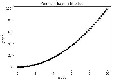
The above shows how easy and quick it is to generate plots from data and to add titles and labels, and to change line styles and markers. Let’s take this a bit further. Seaborn is based on matplotlib and it allows changing styles, color palettes and other decorations very easily. In the next cell, we import Seaborn and define background, grid, fonts and line widths. These definitions have been used to create figures for publications and the line widths and other styles have been selected such that the plots look good when printed.

The best way to use the cell below is to save it separately and then import it. If you plan to use these or some other settings in this same manner, that is what you should do.

#=============================================================
#
# Import Seaborn to make a pretty plot.
#
# Seaborn is excellent for controlling decorations, line widths
# color palettes, etc.
#
#   - Define background for the plot
#   - Define if a grid is used (background)
#   - Define font families
#   - Define line widths
#
# Ideally, this should be put in a separate file and imported, 
# but is included here as an example.
#=============================================================

import seaborn as sns
from matplotlib import rc


sns.set()
sns.set_context("paper", font_scale=1.5, rc={"lines.linewidth": 2.0})

#---- This allows the use of LaTeX + the use sans-serif fonts also for tick labels:

rc('text', usetex=True)
rc('text.latex', preamble=r'\usepackage{cmbright}')

# There are 5 presents for background: darkgrid, whitegrid, dark, white, and ticks
# Define how ticks are placed and define font families

sns.set_style("ticks")
sns.set_style("whitegrid", 
 {'axes.edgecolor': 'black',
 'axes.grid': True,
 'axes.axisbelow': True,
 'axes.labelcolor': '.15',
 'grid.color': '0.9',
 'grid.linestyle': '-',
 'xtick.direction': 'in', 
 'ytick.direction': 'in',
 'xtick.bottom': True,
 'xtick.top': True,
 'ytick.left': True,
 'ytick.right': True, 
 'font.family': ['sans-serif'],
 'font.sans-serif': [
  'Liberation Sans',
  'Bitstream Vera Sans',
  'sans-serif'],})

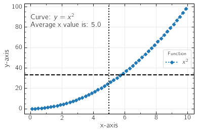
The cell below plots the data using matplotlib with the seaborn settings to make the above plot pretty with nice and consistent fonts, control of tick marks, legends and so on. The line widths were determined in the previous cell so that if the plot is included in an article or thesis, everything should look good. At the end, there is an option to save as png and svg. While png is good for importing plots into Word, LaTeX or LibreOffice, svg (=Scalable Vector Graphics) is scale free. That is, it can be used in posters without loss of resolution and it can be edited (without the need to replot), say, if one wants to change the line type or color. svg files can be edited using the excellent inkscape program (free and available for Windows, Mac and Linux) and then saved to png or any other format if necessary. Note also that svg can be directly imported in LibreOffice files and also in Jupyter Labs/Notebook and on web sites. It’s usually a good idea so save in both formats but if one needs to pick one, svg is a much more flexible choice.

#=============================================================================
#
# Let's make the plot pretty with settings from above.
#
#  - Produces a publication quality plot for an article or thesis.
#=============================================================================

#---- Choose Seaborn colour palette. 
#     This is the only Seaborn piece in this cell, all the rest would work without it.
#     The previous cell does all the decorations and that's what Seaborn did for us.
#
#     More palettes: See: https://seaborn.pydata.org/tutorial/color_palettes.html

sns.set_palette("tab10")

#---- This allows modification of tick positions (& a few other things)

from matplotlib.ticker import (AutoMinorLocator, MultipleLocator)
fig, ax = plt.subplots(1,1)

# Set x and y-minor ticks:

ax.yaxis.set_minor_locator(MultipleLocator(5.0))
ax.xaxis.set_minor_locator(MultipleLocator(1.0))

#---- Plot data. One can use LaTeX for legends (label gets picked up by 
#     the legend part below).
#     Linestyles and markers are more or less the same as in Matlab. See:
#     https://matplotlib.org/2.0.2/api/markers_api.html#module-matplotlib.markers
#     https://matplotlib.org/2.0.2/api/lines_api.html#matplotlib.lines.Line2D.set_linestyle

plt.plot(x_data,y_data, label='$x^2$', linestyle=':', marker='D')

#---- Axis labels and legend:

plt.xlabel("x-axis")
plt.ylabel("y-axis")
plt.legend(title="Function",loc='center right',fontsize='small',fancybox=True)

#---- It's very easy to plot vertical and horizontal lines for example 
#     for the average values or put them in any arbitrary position.
#     Linestyles are the same as in Matlab

plt.axvline(x=np.mean(x_data), color='black', linestyle=':')
plt.axhline(y=np.mean(y_data), color='black', linestyle='--')

#---- You can add text using the coordinate positions (x,y)
#     The example also shows how to concatenate text from extracted data

plt.text(0, 80, 'Curve: $y=x^2$\nAverage x value is: '+str(np.around(np.mean(x_data),decimals=2)), rotation=0)

#---- Uncomment to save. First give a name. Then a high resolution png and svg files are generated

#printfile = 'testplot'
#plt.savefig(printfile+'.svg')
#plt.savefig(printfile+'.png',dpi=300)

#---- Show 

plt.show()

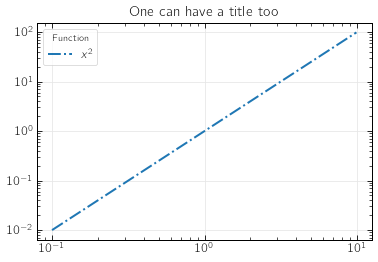
#---- One can plot more so let's generate a log-log plot:

plt.title('One can have a title too')
plt.loglog(x_data,y_data, label='$x^2$', linestyle='-.')
plt.legend(title="Function",loc='upper left',fontsize='small',fancybox=True)

plt.show()

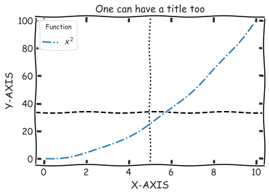
Variation to the theme: plots xkcd style#

Not that this is useful, but it is fun: One can eve plot using the XKCD comics style. To make the plots look more authentic, install the humor sans font (not required, though) from the terminal window using the command sudo apt install -y fonts-humor-sans

Let’s plot the same plot as above.

rc('text', usetex=False)        # Using LaTeX doesn't work with xkcd style so let's turn it off

#-- Note: we use the 'with' since we don't want to make this permanent (only in this context)

with plt.xkcd(scale=1, length=100, randomness=1):   # This turns on the xkcd mode. It has 3 parameters
#with plt.xkcd():                                   # Use default values for the parameters
    plt.xlabel("X-AXIS")
    plt.ylabel("Y-AXIS")
    
    plt.axvline(x=np.mean(x_data), color='black', linestyle=':')
    plt.axhline(y=np.mean(y_data), color='black', linestyle='--')   
    
    plt.title('One can have a title too')
    plt.plot(x_data,y_data, label=r'$x^2$', linestyle='-.') # Note that after turning of LaTeX, this is the way we can have it/
    plt.legend(title="Function",loc='upper left',fontsize='small',fancybox=True)
    
    plt.show()

For more examples and demos, see for example:

Plotting with data from the disk#

The following shows one way of reading data from a file that has data in columns separated by spaces. Seaborn is again used for pretty plots. This also demonstrates numpy and pandas, two very useful modules. This is not very elegant but aim is to demonstrate plotting using data stored in a file, how to use a for loop and how one can get some quick statistics.

We will use two approaches: 1) Direct reading and plotting, and 2) reading the data, converting it to pandas dataframe and then plotting. The second part is shown since pandas dataframe is a very useful (and very commonly used) way of handling data. There are many other ways to plot by calling Seaborn directly, using scatter etc.

Data: It is assumed that data is in $HOME/test_plot/test_data.dat

import pandas as pd
import numpy as np
import matplotlib.pyplot as plt
import os

from helpers import pretty_plots
pretty_plots.pretty_plot(pal='tab10',size='paper')

#---- Get home directory. Demonstrates the module os    
    
home_dir = os.environ['HOME']
print('My home directory is:', home_dir)

#---- Input data: x,y1,y2 data is in this file ----------

data_1 = home_dir+'/test_plot/test_data.dat'

#---- Let's assign arrays and --------------------
#     read the data from the file line-by-line into the variables:
#     Floats are read from a line and appended to the arrays.
#     The data file is opened for reading only.

x, y_1, y_2 =   [], [], []

for line in open(data_1, 'r'):
  values = [float(s) for s in line.split()]
  x.append(values[0])
  y_1.append(values[1])
  y_2.append(values[2])

#---- Let's create a pandas dataframe from the data
#     Note really necessary, but demonstrates pandas

df = pd.DataFrame({
    "time in ns"    : x, 
    "measurement 1" : y_1, 
    "measurement 2" : y_2
})

#---- To write the data as a csv file with the column headers
#     give a name for the out file and uncomment:

#df.to_csv(outfile, index=False)

#---- This is one reason why dataframes are so handy. Let's print it on screen, 
#     easy to see variables and get statistics:

print('\nDataframe:\n')
print(df)

#---- Compute the averages of the two data columns using numpy and print them on screen:

y_1_mean = df['measurement 1'].mean()
y_2_mean = df['measurement 2'].mean()

print('\n')
print(y_1_mean)
print(y_2_mean)
print('\n')

aa=df[['measurement 1','measurement 2']]

#--- print some more statistics

print(aa.dropna().describe())

#---- Create a simple plot of the data in one figure
#     A pretty plot is created below after this one.
#     Note: ax provides a handle to share the axis


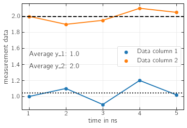
ax = df.plot(x='time in ns',y='measurement 1', s=40, kind='scatter', color='tab:blue', label='Data column 1')
df.plot(x='time in ns',y='measurement 2', ax=ax, s=40, kind='scatter', color='tab:orange', label='Data column 2')
df.plot(x='time in ns',y='measurement 1', ax=ax, kind='line', label='')
df.plot(x='time in ns',y='measurement 2', ax=ax, kind='line', label='')


plt.ylabel("measurement data")
plt.legend(loc='center right')

#---- Plot lines for the average values

plt.axhline(y=y_1_mean, color='black', linestyle=':')
plt.axhline(y=y_2_mean, color='black', linestyle='--')

#---- Plot the average values in the figure.
#     Note: Since LaTeX is enabled, the underscore character needs to be escaped using backslash

plt.text(1, 1.5, 'Average y\_1: '+str(np.around(y_1_mean,decimals=1)), rotation=0)
plt.text(1, 1.35, 'Average y\_2: '+str(np.around(y_2_mean,decimals=1)),rotation=0)


plt.show()

My home directory is: /home/mkarttu

Dataframe:

   time in ns  measurement 1  measurement 2
0         1.0           1.00           2.00
1         2.0           1.10           1.90
2         3.0           0.90           1.95
3         4.0           1.20           2.10
4         5.0           1.02           2.05


1.044
2.0


       measurement 1  measurement 2
count       5.000000       5.000000
mean        1.044000       2.000000
std         0.112606       0.079057
min         0.900000       1.900000
25%         1.000000       1.950000
50%         1.020000       2.000000
75%         1.100000       2.050000
max         1.200000       2.100000

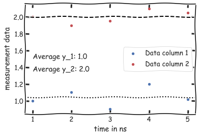
…and of course we can plot this using the xkcd style by reusing the xkcd cell from above:

rc('text', usetex=False)

with plt.xkcd(scale=1, length=100, randomness=1): 
    ax = df.plot(x='time in ns',y='measurement 1', kind='scatter',color='b', label='Data column 1')
    df.plot(x='time in ns',y='measurement 2', ax=ax, kind='scatter',color='r', label='Data column 2')

    plt.ylabel("measurement data")
    plt.legend(loc='center right')

#---- Plot lines for the average values & also write the avg values in the figure

    plt.axhline(y=y_1_mean, color='black', linestyle=':')
    plt.axhline(y=y_2_mean, color='black', linestyle='--')

    plt.text(1, 1.5, 'Average y_1: '+str(np.around(y_1_mean,decimals=1)), rotation=0)
    plt.text(1, 1.35, 'Average y_2: '+str(np.around(y_2_mean,decimals=1)),rotation=0)
    
    plt.show()

A very brief intro to loops and conditionals#

`for` loop#

For loops in python

We already saw an example of this. But here is thefor loop in brief. Note intendation. It is critical.

In example 1, we woop over a range of values, pring out, append values to a list, convert list to a numpy array. Why the last? If/when one needs to perform numerical calculations numpy has lots of optimized routines. As an example, perform an element-wise numpy operation. Why not use lists? Lists are much slower but they are convenient for reading in data and some other stuff.
In example 2, the loop goes over the characters of a string. This is closely related to what was done above when we read lines using a for loop.

#-------------------------------
# Example 1. 

import numpy as np
a = 0                                             # We already used the variable a above so let's initialize it.
b = []                                            # initalize list b and check that it is empty.
print(b)    

for i in range (11,17):
    a = a+i
    b.append(i)                                   # Append values to the list
    print('The value of a is',a,'index:', i)

b_new = np.array(b)                               # Convert b to a numpy array. 
print(b, type(b))                                 # Let's check the original and converted
print(b_new, type(b_new))    
print(np.sqrt(b_new))

[]
The value of a is 11 index: 11
The value of a is 23 index: 12
The value of a is 36 index: 13
The value of a is 50 index: 14
The value of a is 65 index: 15
The value of a is 81 index: 16
[11, 12, 13, 14, 15, 16] <class 'list'>
[11 12 13 14 15 16] <class 'numpy.ndarray'>
[3.31662479 3.46410162 3.60555128 3.74165739 3.87298335 4.        ]

#-------------------------------------
# Example 2.

for i in "Ferme les yeux est imagine-toi par Soprano et Blacko.":
    print(i, end='')  # the part end='' prints without changing line. Comment it out and see.

Ferme les yeux est imagine-toi par Soprano et Blacko.

`while` loops and breaking/stopping a loop#

While loops in python The while loops is used for executing a loop while some (logical) condition is true. Here is also the simples if statement.

#----------------------------------------------
# Example. A simple while loop and a break statement

import numpy as np

x = np.arange(0,10,1)
i = 0
while i < max(x):
    i = i+x[2]
    print(i)
    if i == 4:
        print('Need a break?')
        break

`if` - `elif` - `else` statement#

This is used to test a condition. Note that it is critical to have proper indentation.

#---------------------------------------
# Example. 
#
#   Let's generate random integers between 0 and 100. The argument size gives length of the array (vary it and re-run)

import numpy as np

x = np.random.randint(100,size=(2))
j = 0
for i in x:  
    if x[j] > 6 and x[j] < 10:
        print('Condition 1:',j,x[j])
    elif x[j] > 30 and x[j] < 40:
        print('Condition 2:',j, x[j])
    else:
        print('Condition 3:',j, x[j])
    j = j+1

Condition 2: 0 39
Condition 3: 1 58

What was not covered#

The above covers the basics and provides a starting point for being able to produce and analyze data. The main thing that was not covered is object oriented programming. For those who are interested, here is some further reading:

Object-Oriented Programming (OOP) in Python 3

Molecular Dynamics Simulations

Brief introduction to Python

Contents

Brief introduction to Python#

Python, what is it good for?#

Python vs other languages#

Python basics – the necessary prerequisites#

How to use the rest of this section#

Install Python virtual environment#

Getting help#

Variables and data types#

Keywords, variable names and first touch of `import`#

Integers & floats#

Strings and slicing operator#

Lists#

Tuples - ordered immutable lists of elements#

Dictionaries#

Combined variables#

Checking who’s who: `type`, `len`, `id`#

Type conversion#

Operators#

Import modules#

Plotting in python#

Variation to the theme: plots xkcd style#

Plotting with data from the disk#

A very brief intro to loops and conditionals#

`for` loop#

`while` loops and breaking/stopping a loop#

`if` - `elif` - `else` statement#

What was not covered#

Molecular Dynamics Simulations

Brief introduction to Python

Contents

Brief introduction to Python#

Python, what is it good for?#

Python vs other languages#

Python basics – the necessary prerequisites#

How to use the rest of this section#

Install Python virtual environment#

Getting help#

Variables and data types#

Keywords, variable names and first touch of import#

Integers & floats#

Strings and slicing operator#

Lists#

Tuples - ordered immutable lists of elements#

Dictionaries#

Combined variables#

Checking who’s who: type, len, id#

Type conversion#

Operators#

Import modules#

Plotting in python#

Variation to the theme: plots xkcd style#

Plotting with data from the disk#

A very brief intro to loops and conditionals#

for loop#

while loops and breaking/stopping a loop#

if - elif - else statement#

What was not covered#

Keywords, variable names and first touch of `import`#

Checking who’s who: `type`, `len`, `id`#

`for` loop#

`while` loops and breaking/stopping a loop#

`if` - `elif` - `else` statement#