Review of thermodynamics

Thermodynamics can be defined as the study and science of heat. Importantly, there is no equation of motion in thermodynamics, and it is a macroscopic and phenomenological theory.

The following provides a brief review of some of the important concepts.

Thermodynamics

Thermodynamics is a macroscopic theory of state variables of a given physical system. The leading concepts in thermodynamics are energy, entropy and absolute temperature.

There is often some confusion regarding what is the relation between thermodynamics, kinetic theory (of gases) and the ensemble theory of statistical mechanics.

1. Thermodynamics is a macroscopic theory, it doesn’t contain any microscopic information. The theory is largely due to Sadi Carnot who published it in 1824.

2. Kinetic theory (of gases) is microscopic theory of molecular distributions. It was originally developed for dilute gases by James Clerk Maxwell and Ludwig Boltzmann in the 1870’s.

3. Ensemble theory of statistical mechanics. Here, the core concept is the microscopic partition function: All thermodynamic information can be derived from the partition function. The theory was formulated by Josiah Willard Gibbs around 1902.

When analyzing trajectory data from simulations, we often compute thermodynamic quantities using distributions and microscopic data: Statistical mechanics is the key to analyzing simulation data. We will give a more precise definition for statistical mechanics below after reviewing some of the basic concepts in thermodynamics.

Sadi Carnot, one of the founders of modern thermodynamics

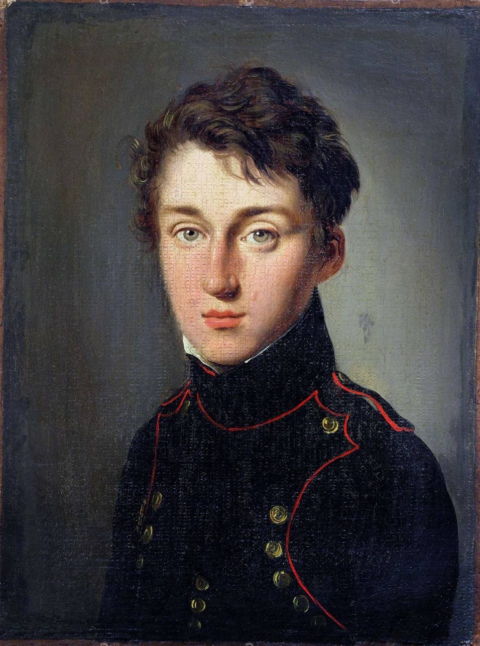
Sadi Carnot is one of the pioneers of thermodynamics. He was military engineer educated in the famous École Polytechnique. His 1824 book “Réflexions sur la puissance motrice du feu et sur les machines propres à développer cette puissance” (Reflections on the Motive Power of Fire and on Machines Fitted to Develop that Power) is a fundamental work in thermodynamics and it contains the second law of thermodynamics. His work was drive by a very practical goal: Carnot hoped to discover the general operating principles of steam engines. The book remained practically ignored for over 20 years until became an inspiration to scientists in the mid 1850’s - those 20 years cover the time of the so-called second cholera pandemic of 1826-1837. Carnot died of cholera at the young age of 36 in 1832 while studying the cholera epidemic. Very little of his originals works has been preserved since most of his papers and belongings were destroyed as was the common practise in the case of cholera victims.

After the pandemic, Émile Clapeyron who survived the pandemic and had been Carnot’s classmate at École Polytechnique put Carnot’s work in a mathematical form using differential equations. Clapeyron’s work was groundbreaking and it inspired scientists such as Rudolf Clausius and William Thomson (also know as Lord Kelvin). As a direct consequence of Clapeyron’s work, Lord Kelvin used Clapeyron’s mathematical formalism to define the absolute temperature scale.

“Say little about what you know and nothing at all about what you don’t know. When a discussion degenerates into a dispute, keep silent. Do not do anything which the whole world cannot know about.”

• Sadi Carnot, “Rules of Conduct”.

Laws of thermodynamics

Below is a very brief review of the laws of thermodynamics. Please notice that there are different but equivalent ways to state each of the laws.

Zeroth law: Thermal equilibrium

This law is formulated by Sir Ralph Fowler who was the supervisor of three physics Physics Nobel Laureates, Paul Dirac, Subrahmanyan Chandrasekhar and Sir Neville Mott.

The most common way of stating the zeroth law is the following by Edward Guggenheim:

“If two systems are both in thermal equilibrium with a third system, then they are in thermal equilibrium with each other.”

Fig. 10 Illustration of the zeroth law of thermodynamics. If systems 1 and 2 have the same temperature as systems 2 and 3, then systems 1 and 3 must also have the same temperature.

First law: Energy conservation

The first law of thermodynamics is most often stated as “The total energy of an isolated system remains constant.”

\[ d U = {\large \it{ đ}} Q - {\large \it{ đ}}W \]

where

• \(d U\) is the change in internal energy

• \( {\large \it{ đ}} Q\) is heat added into the system

• \({\large \it{ đ}}W\) is work done by the system

If the process is reversible, the differentials \( {\large \it{ đ}} Q\) and \({\large \it{ đ}}W\) are exact (see: exact differential) and they are given as

• \(dW = pdV\)

• \(dQ = TdS\)

Second law: Irreversibility

The most compact way of stating the second law of thermodynamics is

\[ \Delta S \ge 0. \]

The case of \(\Delta S = 0\) corresponds to a reversible process.

The perhaps most common and descriptive way to state the second law is the formulation by Rudolf Clausius, one of the founders of modern thermodynamics, that heat does not spontaneously pass from a colder to a hotter body.

Third law: Absolute zero

The third law is sometimes called Nernst’s law after Walther Nernst who formulated what is called the Nernest heat theorem. Nernst was awarded the 1920 Nobel Prize in Chemistry “in recognition of his work in thermochemistry”.

The most compact way of stating the third law is:

\[ \lim_{T \rightarrow 0} S(T) = 0. \]

This states that at zero temperature, the system must be at its ground state. In terms of Boltzmann’s formula,

\[ S = k_\mathrm{B} \ln S \]

this means that there is only one single possible microstate since \(\ln (1) = 0.\) Notice that a quantum system still exhibits zero-point entropy.

State variables

Thermodynamics deals with state variables, that is, macroscopic variables that describe the whole system. This is different from statistical mechanics that uses microscopic variables.

The extensive and intensive variables have also a very important relation: For each extensive variable there is a conjugate intensive variable and (vice versa). For example, temperature and entropy and conjugate variables as are volume and pressure. This property is very important when discussing free energies. IN addition, state variables are meaningful only when the system is in equilibrium.

It is also noteworthy that in a typical situation, there are only a few independent state variables. When the state variables are known, they provide a complete description of the thermodynamic state of the system.

The central paradigm of thermodynamics

The central paradigm of thermodynamics

The paradigm of thermodynamics is to derive an equation of state in terms of the state variables. The equation of state is some continuous but not necessarily analytic function of the form

\[ g(p,V,T,...) = 0 \]

Why is the equation of state so important? Once the equation of state is known, it can be used to derive experimentally measureable response functions such as compressibility, heat capacity and so on. This also works the other way around: Experimental data can be used to help to construct an equation of state. An equation of state should also be able to describe phase transitions, that is, it can be used to construct a phase diagram for the system. To be able to provide a complete thermodynamic description of a system, one needs to know 1) the equation of state and 2) the relevant thermodynamic potential. Both of them are described by the state variables.

Thermodynamic potentials

Here, we will only review the cases in which the system has a constant number of particles in it (our MD simulations have a fixed number particles), that is \(dN = 0\). Note that in equilibrium, free energy is minimized and that is different from minimizing energy. How to choose the correct thermodynamic potential? It depends on what the natural variables are, that is, if the system is constant energy, pressure, temperature, particle number and so on.

The most important thermodynamic potentials and their natural variables are:

Name	Equation
Helmholtz free energy:	\(F \equiv F(T,V) = U - TS = -PV - TS\)
Internal energy:	\(U \equiv U(S,V) = H-PV = TS-pV \)
Enthalpy:	\(H \equiv H(p,S) = U+pV = pV + TS\)
Gibbs’ free energy:	\(G \equiv G(p,T) = F+pV = PV - TS\)

The corresponding differentials are

\[\begin{split} dF & = -pdV - SdT & = \left( \frac{\partial F}{\partial V} \right)_T dV + \left( \frac{\partial F}{\partial T} \right)_V dT \\ dU & = -pdV + TdS & = \left( \frac{\partial U}{\partial V} \right)_S dV + \left( \frac{\partial U}{\partial S} \right)_V dS\\ dH & = Vdp + TdS & = \left( \frac{\partial H}{\partial p} \right)_S dp + \left( \frac{\partial H}{\partial S} \right)_p dS\\ dG & = -SdT + VdP & = \left( \frac{\partial G}{\partial T} \right)_p dT + \left( \frac{\partial G}{\partial p} \right)_T dp % \Psi \end{split}\]

Important equations of state

Now that we have defined the central paradigm of thermodynamics, state variables and thermodynamic potentials, let’s briefly review some of the equations state.

Ideal gas

The ideal gas is defined as a monatomic low-density gas that consists of point-like (zero size) non-interacting particles. It is further assumed that the inter-atomic collisions are fully elastic and conserve energy, and that there is no exchange of energy or particles with the surroundings. These conditions mean that the total energy of the system is conserved. It is further assumed that the gas is in equilibrium at temperature \(T\).

The atoms move at speed \(v\),

\[ v^2 = v_x^2 + v_y^2 + v_z^2 \]

Since the gas in equilibrium, the system has both translational and rotational invariance meaning that the atoms have equal probability in moving in any direction with the average speed being equal

\[ \langle v_x^2 \rangle = \langle v_y^2 \rangle = \langle v_z^2 \rangle . \]

Since all the components are equal, then each of them contributes one third to the average speed, that is,

\[ \langle v \rangle = 3 \times \langle v_x^2 \rangle = 3 \times \langle v_y^2 \rangle = 3 \times \langle v_z^2 \rangle \]

or

\[ \frac{ \langle v^2 \rangle}{3} = \langle v_x^2 \rangle = \langle v_y^2 \rangle = \langle v_z^2 \rangle \]

Since there are no interactions, all the energy is in the form of kinetic energy. With this information, we can write the total energy for a system of \(N\) atoms (of mass \(m\)) as the sum of the individual kinetic energies as

(11)\[\begin{equation} E_\mathrm{tot} = E_\mathrm{k} = \sum_{i=1}^N \frac{1}{2}m \langle v^2 \rangle = \frac{1}{2}N m \langle v^2 \rangle = \frac{3}{2}N m \langle v_x^2 \rangle % = \frac{3}{2} Nk_\mathrm{B} T \end{equation}\]

The last equality follows from the equation above (it can be equally well be written in terms of either the \(y\)- or the \(z\)-component.

We have now several state variables: kinetic energy (\(E_\mathrm{tot}=E_\mathrm{kin}\)), temperature (\(T\)), pressure (\(p\); follows from the elastic collisions of the atoms with the walls of the container) and the number of particles (\(N\)). How can we get the equation of state? We can use a heuristic way and analyze the properties and quantities:

• Heuristic derivation: We have an extensive quantity, volume, and two intensive quantities, pressure and temperature. We also have the total energy which is a state function and depends on the system size. We also know that volume and pressure and conjugate variables, and that a product of two conjugate variables has units of energy (check by multiplying \(p\) and \(V\)). We also know that energy is given as \(k_BT\) or alternatively as \(nR.\) By matching units (this is an example of dimensional analysis), we can propose the following:

\[ pV = Nk_\mathrm{B}T. \]

The above was a heuristic example using dimensional analysis. It is possible to derive the ideal gas law in a more rigorous manner, but for that we need a connection between the microscopic properties and thermodynamics. That connection is provided by statistical mechanics.

The equation of state for an ideal gas can be given in the following two equivalent forms,

\[\begin{split} pV & = Nk_\mathrm{B}T \\ pV & = n R T \end{split}\]

where \(p\) is pressure, \(V\) is volume, \(N\) is the number of particles, \(k_\mathrm{B}\) the Boltzmann constant, \(T\) temperature, \(n\) the number of moles and \(R\) the gas constant. The Boltzmann constant is \(k_\mathrm{B} = 1.380649 \times 10^{−23}\) J/K, and the gas constant can be given using \(k_\mathrm{B}\) and Avogadro’s constant \(N_\mathrm{A}\) as \(R = N_\mathrm{A} k_\mathrm{B} = 8.314\) J/(K mol).

As discussed above, to be able to provide a complete thermodynamic description of a system, one needs to know 1) the equation of state and 2) the relevant thermodynamic potential. Here we have both of them and we could analyze all thermodynamic properties of the system. The ideal gas is an exception as this is not the case for more realistic systems

Despite being simple, the ideal gas is still a very useful concept. The ideal gas equation of state is, however, not capable of describing any kind of phase transitions. This is due to the assumptions that were made: Real particles are not of zero size and point-like and real particles do interact. The van der Waals equation of state adds those components.

Fig. 11 In a real gas particles have a finite size, they occupy a finite volume. In an idea gas particles are point-like (diameter is zero) and there are no interactions between them.

Van der Waals equation of state

The van der Waals equation of state is the simplest equation of state that can describe a phase transition and it was originally proposed by Johannes Diderik van der Waals in his PhD thesis in University of Leiden (the Netherlands) in 1873. His thesis was written in Dutch and titled “Over de Continuïteit van den Gas- en Vloeistoftoestand” (on the continuity of the gaseous and liquid state). He was awarded the Nobel Prize in Physics in 1910 “for his work on the equation of state for gases and liquids.” Van der Waals’ contribution to the molecular theory matter are very broad as manifested by terms such as van der Waals forces, van der Waals radius for sizes of molecules, and van der Waals surface used in visualization of molecules.

As van der Waals’ thesis title indicates, the theory was originally developed to describe a vapour-liquid phase transition (and it cannot describe liquid-solid transitions). The theory describes an interacting gas consisting of atoms of finite size. For a non-rigorous derivation, the ideal gas law can be taken as a starting point. The right hand side in \(pV = nRT\) has \(n\), \(R\) and \(T\). Those are quantities that don’t need any corrections, but the left hand side is different: 1) If particles have a finite size, the whole volume is no longer available for them. How much the free volume is reduced depends on the size and number of the particles. 2) If particles interact, pressure will be different from that of ideal gas; the pressure is reduced due to the attractive van der Waals interactions. The magnitude of the change depends on the density of the particles, but those are the two terms that will be modified.

The van der Waals equation of state can be written as

(12)\[\begin{equation} \left( p + a \frac{N^2}{V^2} \right) \left( V-bN \right) = N k_\mathrm{B}T \end{equation}\]

where \(a\) and \(b\) are constants. Although the above heuristic argument suggests the origin of the two constants, they have no direct correspondence to measurable quantities. There has been efforts, however, to relate them to physical observables[1, 2].

The above can also be written in the form

(13)\[\begin{equation} p = \frac{N k_\mathrm{B}T}{V-bN} - a \frac{N^2}{V^2}. \end{equation}\]

This form shows immediately that the first term is the ideal gas term amended with the finite size of particles and the second term is a reduction in pressure caused by the particle-particle interactions; as the volume increases, the gas becomes dilute, this term becomes less and less important and the behavior approaches that of an ideal gas.

Let’s look at the correction terms with some more detail. The correction to pressure depends on \((N/V)^{2}\). This may seem odd in the first place, but there is a good reason: The particles interact and the interaction are assumed to be pair-wise 2-body interactions. The probability for two particles to be to interact attractively \(\sim (N/V)^{2}\). When there is an attractive interaction, the pressure that they extert on the walls of the container is reduced and hence the negative sign in the latter formulation.

The finite size of atoms leads to short-range repulsion since atoms cannot overlap. The second new term, \(Nb\), is correction to the volume due to finite size of atoms (or molecules). This volume is not accessible for other molecules (due to Pauli exclusion principle). Thus, the volume that is available in a system, the free volume, containing \(N\) atoms is reduced by \(Nb\): \(V_\mathrm{free} = V - Nb\).

In is also noteworthy that at the time when van der Waals proposed his theory, the atomic theory of matter was generally not accepted and several prominent scientist vehemently opposed the molecular view of matter. The most notable proponents of this view were Wilhelm Ostwald, the 1909 Nobel Laureate in Chemistry (“in recognition of his work on catalysis and for his investigations into the fundamental principles governing chemical equilibria and rates of reaction”) and Ernst Mach (the Mach number is named after him).

Instead of the heuristic justification above, the van der Waals equation of state can be derived from statistical mechanics.

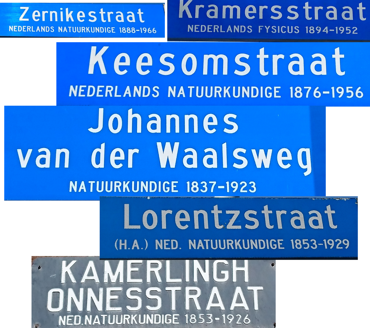
Fig. 12 Some of the many science-related streets signs in Eindhoven, the Netherlands, showing appreciation for science, amongst them van der Waals Street. These are the scientists: Frits Zernike, Nobel in Physics in 1953; Hans Kramers; Willem Keesom; Johannes Diderik van der Waals, Nobel Prize in Physics in 1910; Hendrik Lorentz, Nobel Prize in Physics 1902; Heike Kammerlingh Onnes, Nobel Prize in Physics in 1913 for the discovery of superconductivity.

Virial equation of state

The final equation of state that we discuss is the virial equation of state. It is very useful for many reasons and in this context is provides a connection between simulations, experiments and also the van der Waals equation of state. Historically, the virial equation of state was formulated by Heike Kammerlingh Onnes who was awarded the Nobel Prize in Physics in 1913 for the discovery of superconductivity. Onnes’ studies of the equation of state and the development of the virial equation of state were also critical in the discovery of superconductivity. On a side note, one of Onnes’ students, Pieter Zeeman was also awarded the Nobel Prize in Physics (for the Zeeman effect).

The basic idea is to use the number density, \(\rho = N/V\) as an expansion variable and use power series to expand the ideal gas equation of state. Since power series converges only when the expansion parameter is small, the virial expansion works, strictly speaking, only for dilute gases. The idea of using such an expansion that it is essentially a perturbation approach and we are expanding around a reference state. This is also reflected in the expansion parameter: it has to be small since the expansion is done in the proximity of the reference state and the expansion must converge and each successive term should be small correction to the previous ones. This approach is used in many other fields, espcially in quantum mechanics. Let’s see how that works:

\[\begin{split} pV & = Nk_\mathrm{B} T \\ p & = p(N,V,T) = k_BT \frac{N}{V} \\ p & = p (\rho, T) = k_BT \rho \\ p & = k_\mathrm{B}T \sum_{n=0}^{\infty} B_n \rho^n \\ p & = k_\mathrm{B}T \left[B_0 + B_1(T) \rho + B_2(T) \rho^2 + B_3(T)\rho^3 + \dotsb \right] \\ %p & = k_\mathrm{B}T \left[ \rho + B_2(T) \rho^2 + B_3(T)\rho^3 + \dotsb \right] \end{split}\]

Let’s look at the expansion coefficients \(B_i(T)\). Physically, we have to obtain the ideal gas law when the system becomes infinitely dilute, that is, when \(\rho \rightarrow 0\) such that both \(N\) and \(V\) remain finite.; this is called the thermodynamic limit. This condition means that \(B_0 = 0\) and \(B_1(T) = 1\). At that limit the higher order terms must vanish since the gas becomes and ideal gas. We can now re-write the above as

\[\begin{split} p & = \rho + k_\mathrm{B}T \sum_{n=2}^{\infty} B_n \rho^n \\ p & = k_\mathrm{B}T \left[\rho + B_2(T) \rho^2 + B_3(T)\rho^3 + \dotsb \right] \\ \end{split}\]

To go further, let’s ask the question is the physical interpretation of these expansion coefficients. As discussed above, they represent corrections to the references state. These corrections originate, at least qualitatively, from molecular interactions. Take the limit \(\rho \rightarrow 0\) gave us the situation with no particle-particle interactions. Thus, including pairwise interactions (2-body interactions) is the first correction as the density becomes larger: Pairs of particles start to interact and thus the term \(B_2(T)\) is pair-interaction term. Similarly, the higher-order terms arise from 3-body interactions, 4-body interactions and so forth. The coeffiecients are called the virial coefficients and they depend on the nature of the gas and the interactions present in the system. However, to provide a more precise connection to molecular interactions, statistical mechanics is needed.

We have now established qualitatively that the coefficients include information about molecular interactions.

Digression: Power series

Power series around point \(x_0\) can be defined the following way,

\[ f(x) = \sum_{n=0}^{\infty} a_n (x-x_0)^n = a_0 + a_1 (x-x_0) + a_2 (x-x_0)^2 + \dotsb + a_k (x-x_0)^k + \dotsb \]

where the constants \(a_n\) are independent of \(x\). When \(x_0 =0\), this reduces to the familar form

\[ f(x) = \sum_{n=0}^{\infty} a_n x^n = a_0 + a_1 x + a_2 x^2 + \dotsb + a_k x^k + \dotsb + \]

Convergence must be tested by, for example, d’Alembert’s ratio test. In addition, the function that is expanded must be continous in the domain of (uniform) convergence.

Review of statistical mechanics

There is sometimes confusion as what is thermodynamics vs. statistical mechanics. Thermodynamics uses state variables and it doesn’t provide a molecular picture. Thermodynamics is phenomenological. Statistical mechanics provides that molecular picture and answers the why in thermodynamics. From the technical standpoint, statistical mechanics applies statistics and probability to the microscopic molecular properties described using classical and quantum mechanics.

Statistical mechanics vs thermodynamics

The object of statistical mechanics is to provide the molecular theory for equilibrium processes of macroscopic systems.

Statistical mechanics answers the why in thermodynamics.

Equilibrium

When we discussed simulations, we talked about equilibration but we didn’t defined what exactly it is. Equilibrium is one of the most fundamental and important concepts. Importantly, thermodynamics and statistical mechanics are valid only in equilibrium. There are fields called non-equilibrium thermodynamics and non-equilibrium statistical mechanics but those theories describe processes in which there is heat transport (or other currents), friction, external forces and so on. Such theories are beyond the scope of this course.

Qualitatively, a system in equilibrium must fulfill the conditions that: 1) there can be no macroscopic flows or changes going on in the system and 2) the system possesses no history. The latter means that once the system has reached equilibrium, it carries no information how it got there, that is, it is impossible to tell what was the initial state of the system. While this may sound abstract (even meaningless in the first place), this property is very important and practical: Foe example, it is often very difficult to determine if the system has reached equilibrium (the short simulations that we have performed are, technically speaking, not in equilibrium). One way to test it is to run multiple simulations (sometimes called replica simulations) of the same system but starting from different initial conditions. For example, one could run 5-10 independent simulations. If the systems reached equilibrium, the results, when analyzed, should all be within the margin of error of each other. This is indeed what is typically done.

Let’s now provide a more formal definition for equilibrium: A system is in thermodynamic equilibrium when the following three macroscopic criteria are fulfilled:

1) Mechanical balance: No net forces or torques are present:

\[\begin{split} \sum_i \vec{F}_i & = 0\\ \sum_i \overline{\overline{\tau}}_i & = 0 \end{split}\]

2) Thermal balance: thermodynamic variables are time-independent. This means that there is no net heat, or other comparable flows in the system:

(14)\[\begin{equation} \frac{\partial p}{ \partial t} = \frac{\partial V}{\partial t} = \dotsb = 0 \end{equation}\]

3) Chemical balance: No macroscopic particle currents are present:

(15)\[\begin{equation} \mu_i = \mathrm{constant} \end{equation}\]

In equilibrium the thermodynamic potentials (Helmholtz free energy, Gibbs free energy, enthalpy, internal energy and the grand potential) are minimized. In addition, entropy is maximized for isolated systems. One should also notice the following: Thermodynamic state variables are macroscopic and do not fluctuate. Microscopic quantities used in statistical mechanics do fluctuate, thermal fluctuations are always present (when \(T \ne 0\) K).

Importantly, if the system is not in equilibrium, the formalisms of thermodynamics and statistical mechanics cannot be applied. If one does that, the results are wrong and meaningless. This is why one must always pay a lot of attention and perform analyses, and often additional simulations to ensure the system under study has reached its equilibrium state.

Le Chatelier’s principle: For a system in stable equilibrium, any spontaneous (= not caused by external forces or fields) change leads to processes that restore the equilbrium.

Fig. 13 The idea of Le Chatelier’s principle. Left: If the system is perturbed from its free energy minimum by thermal fluctuations, the equilibrium state will be restored. Middle: If the system is in a metastable state and the thermal fluctuations are small, the system will return to that same metastable state. Right: If one waits long enough, there will be large thermal fluctuataions (they are Gaussian distributed so there will be such fluctuations if one waits long enough), the system will eventually find the the global equlibrium. This is also an example of negative (restoring) feedback. Green sphere: the system’s state described by state variables.

Boltzmann distribution

Maxwell-Boltzmann distribution

Below are two videos showing how teh Maxwell-Boltzmann distribution emerges spontanously during a particle simulation. The two systems are identical in the number of particles, but the system with larger particles has a diameter that about 2.5 times larger than the one with smaller particles. The simulations have hard walls with fully eleastic energy-conserving collisions and the simulation is performed in 2-d for speed. In both cases the two systems start from random configuration of particles and veolcities. Due to the larger size of particles in the second simulation, there are more collisions and the Maxwell-Boltzmann distribution emerges faster. The orange line shows the analytical form of the Maxwell-Boltzmann distribution, the blue line shows the averaged distribution (averaging starts after 500 time steps) and the histogram shows the instantanous distribution.

Permutations and combinations

Permutations, combinations and Stirling’s forumula

Permutation gives the number of distinct arrangements of \(N\) different objects

Combination gives the number of arrangements of \(N\) objects of which \(n\) is chosen at a time.

(16)\[\begin{equation} N! = N \times (N-1) \times \dotsb \times 1 \end{equation}\]

Bibliography

1

Sam P. de Visser. Van der waals equation of state revisited: importance of the dispersion correction. The Journal of Physical Chemistry B, 115(16):4709–4717, apr 2011. doi:10.1021/jp200344e.

2

Georgios M. Kontogeorgis, Romain Privat, and Jean-Noël Jaubert. Taking another look at the van der waals equation of state–almost 150 years later. Journal of Chemical & Engineering Data, 64(11):4619–4637, aug 2019. doi:10.1021/acs.jced.9b00264.