Interactions

We have already defined classical molecular dynamics as follows:

Definition of Molecular Dynamics (MD)

Molecular Dynamics is the evolution of Newton’s equations motion in time. In short, the problem is simply to solve numerically F=ma.

Using Newtonian mechanics means that we do not consider any quantum mechanical phenomena. The practical consequences include that classical MD doesn’t have electrons and cannot describe chemical reactions.

Basic concepts: the Hamiltonian

Typically, the system is described by a model Hamiltonian that depends on the degrees of freedom the system has. The Hamiltonian expresses the total energy of an isolated system as a function of coordinates and momenta. In the following, we denote the coordinates by \(\vec{q}\) and the momenta by \(\vec{p}\). The Hamiltonian, \(\mathcal{H} \equiv \mathcal{H}(\vec{q}, \vec{p})\), is defined as the sum of the kinetic (\(T\)) as

(1)\[\begin{equation} \mathcal{H} = T + V. \end{equation}\]

It is worth remembering that in the Lagrangian formulation of classical mechanics, the energy function (the Lagrangian) is defined as the difference between the kinetic and potential energies, that is, \(\cal{L} = T-V\). The Hamiltonian and the Lagrangian are related to each other via a Legendre transform.

Conservation of energy

It is important to notice that Hamilton’s equations of motion conserve the total energy of the system. Conservation of energy can be simply expressed as

(2)\[\begin{equation} \frac{d \mathcal{H}}{dt} = 0, \end{equation}\]

in other words, \(\mathcal{H}(\vec{q}, \vec{p}) = \mathrm{constant}\).

This has also some very pragmatic consequences: The conservation of energy means that any MD simulation (without the addition of thermostats and such), must obey this. That is, the energy of the system must remain constant throughout the simulation. This is a strict requirement and can/should be used to check that the simulation is performing correctly. If energy is either decreasing or increasing, there is something (seriously) wrong with the simulation.

Let’s discuss this a bit further. We know from classical mechanics that conservative forces do not depend on time, only the position. Conservative forces have to fulfill any of the following equivalent conditions,

1. \( \nabla \times \vec{F} = 0\).

2. \(W = \oint_C \vec{F} \cdot \vec{r}= 0\), where \(W\) is work.

3. \(\vec{F} = - \nabla U\), where \(U\) is the potential.

The Lennard-Jones potential

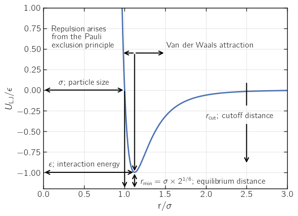
The Lennard-Jones (LJ) potential is the most common way of describing non-bonded (non-electrostatic) particle-particle interactions. The LJ potential can be written as

(3)\[\begin{equation} U_\mathrm{LJ} = 4 \epsilon \left[ \left( \frac{\sigma}{r} \right)^{12} -\left( \frac{\sigma}{r} \right)^6 \right], \end{equation}\]

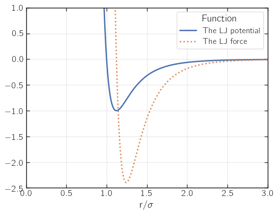
where \(\epsilon\) is the value of the potential at its minimum and \(\sigma\) is related to the atomic diameter (we’ll elaborate on that later). The LJ potential and some of its main features are plotted below.

It is important to notice that although the LJ potential is classical, it has a quantum mechanical origin. The repulsive \(r^{-12}\) term cannot be derived from first principles and, in principle, any rapidly diverging term for \(r \rightarrow 0\) is possible. The above form is the most commonly used one. Although the term cannot be derived analytically, it has its origin in the Pauli exclusion principle, i.e., it has a quantum mechanical origin.

The attractive \(r^{-6}\) term can be analytically derived using the Lifshitz theory (beyond this course). Physically, it arises from the spontaneous fluctuations of the electric dipole moment caused by the motions of the electrons: An atom causes a fluctuation in the electron clouds of the neighboring atoms and vice versa giving rise to dipole and multipole moments. This is why it is sometimes called the dispersion interaction. It is also important to notice that the van der Waals \(r^{-6}\) term is always attractive.

The van der Waals force (\(r^{-6}\) term) has three contributions:

1. Keesom force: Interactions between permanent charges and multipoles

2. Debye force, also called polarization: Forces between a permanent multipole and an induced multipole.

3. London forces, also called London dispersion interactions: These are instantaneous dipole–induced dipole forces.

Averaging over random orientations yields a \(r^{-6}\) term for each of the above.

Let’s now return to the \(\sigma\) parameter. As the figure shows, \(\sigma\) gives the distance at which the interaction between two particles is zero. If the particles are identical, \(\sigma\) is then the diameter of the particle. The situation is more complex when the particles are not identical, and we will return to this matter later.

The LJ potential is used in essentially all classical level molecular modeling, and it is a surprisingly good fit (albeit with caveats) when only two-body interactions are important. It is important to notice that the LJ potential is short-ranged.

The Lennard-Jones potential is named after Sir John Lennard-Jones.

Sir John Lennard-Jones

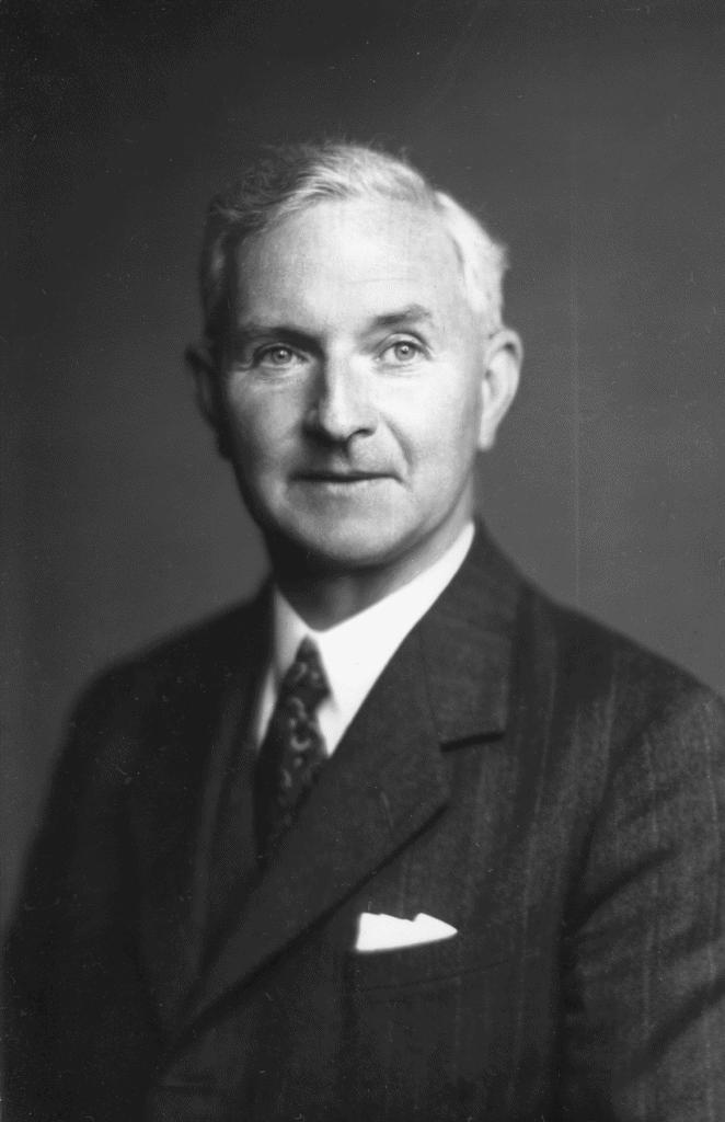
Sir John Lennard-Jones was the PhD supervisor of Sir John Pople who shared 1998 Nobel Prize in Chemistry with Walter Kohn. Lennard-Jones’ PhD supervisor was Sir Ralph Fowler - three of his PhD students became Physics Nobel Laureates, namely Paul Dirac, Subrahmanyan Chandrasekhar and Sir Neville Mott.

The Lennard-Jones potential used in almost all classical molecular dynamics simulations is named after him and he was the first person in the world to hold a Chair of Theoretical Chemistry(U. Cambridge 1932)[].

Picture credit: Copyright Computer Laboratory, University of Cambridge. Reproduced by permission. Creative Commons License.

Cutoff

To be useful in simulations, we have to introduce a cutoff, \(r_\mathrm{cut}\), for the LJ potential. This cutoff leads to discontinuity in the potential and sometimes the potential is shifted to be zero at \(r_\mathrm{cut}\).

Dimensionless units

It is very common to express (and use) the LJ potential using reduced, or dimensionless, units. This can be done by noticing that the LJ potential,

(4)\[\begin{equation} U_\mathrm{LJ} = 4 \epsilon \left[ \left( \frac{\sigma}{r} \right)^{12} -\left( \frac{\sigma}{r} \right)^6 \right], \end{equation}\]

has only two parameters, \(\sigma\) and \(\epsilon\). In addition, particle mass (\(m\)) is a free parameter.

LJ parameters

1. \(\sigma\): unit of length

2. \(\epsilon\): unit of energy

3. \(m\): unit of mass.

Using these, we can define the dimensionless length and potential as

\[ r^* \equiv \frac{r}{\sigma} \]

and

\[ u^* \equiv \frac{U_\mathrm{LJ}}{\epsilon} \]

Why would this be a good idea? There are several reasons. A practical reason is that instead of using atomic dimensions, with reduced units all the dimensions are of the order of unity making the simulations numerically more stable. There is also a deeper reason: Using the reduced units transforms the LJ potential to the form

\[ U_\mathrm{LJ} = \epsilon u^*(\sigma/r). \]

This means that all the systems that can be described by the above formula follow the same equation of state. Thus, the Law of Corresponding States applies. From the practical point of view, we can then simulate all such systems setting \(\sigma = 1\), \(\epsilon =1\) and \(m=1\).

Using the above reduced units, we can give the dependent quantities in terms of the new variables. For example,

• temperature: \(\frac{k_BT}{\epsilon}\)

• density: \(\rho \sigma^3\)

• pressure: \(\frac{p \sigma^3}{\epsilon}\)

• force: \(\frac{F \sigma}{\epsilon}\)

• time: \(t\,\sqrt{\frac{\epsilon}{m \sigma^2}}\)

• surface tension: \(\frac{\gamma \sigma^2}{\epsilon}\)

• velocity: \(v \sqrt{\frac{m}{\epsilon}}\)

In addition, it is common to set \(k_\mathrm{B} = 1\) which further simplifies the above.

away that both good and bad solvent conditions can be be modelled. Good solvent conditions can be modelled by the purely repulsive so-called truncated and shifted Lennard-Jones potential,

The Lennard-Jones force

Using the Hamiltonian formulation of mechanics, the equations of motion are written as a set of first-order differential equations

(5)\[\begin{equation} \vec{F}(r_{ij}) = - \nabla U(r_{ij}). \end{equation}\]

Let’s see this through a practical example. With the help of the chain rule, the force that atom 2 exerts on atom 1 can be written as

\[\begin{align*} \vec{F}_{21} & = - \nabla_{\vec{r}_1} U_\mathrm{LJ}(r_{12}) \\ & = - \left [ \frac{\partial U_\mathrm{LJ}(r_{12})}{ \partial x_1} \hat{i} + \frac{\partial U_\mathrm{LJ}(r_{12})}{ \partial y_1} \hat{j} + \frac{\partial U_\mathrm{LJ}(r_{12})}{ \partial z_1} \hat{k} \right] \\ & = - \frac{dU_\mathrm{LJ}(r_{12})}{dr_{12}} \left[ \frac{\partial r_{12}}{\partial x_1} \hat{i} + \frac{\partial r_{12}}{\partial y_1} \hat{j} + \frac{\partial r_{12}}{\partial z_1} \hat{k} \right] \end{align*}\]

This can be simplified by remembering that \(r_{12} = |\vec{r}_{12}| = \sqrt{(x_2-x_1)^2 + (y_2-y_1)^2 + (z_2-z_1)^2 }\) and that

\[\begin{align*} \vec{r}_{12} & = (x_2-x_1) \hat{i} + (y_2-y_1) \hat{j} + (z_2-z_1) \hat{k} \\ &= x_{12} \,\hat{i} + y_{12} \, \hat{j} + z_{12} \,\hat{k} \end{align*}\]

Using these yields

(6)\[\begin{equation} \vec{F}(r_{21}) = -\frac{dU_\mathrm{LJ}(r_{12})}{dr_{12}} \frac{1}{|\vec{r}_{12}|} \left[ x_{12}\,\hat{i} + y_{12}\,\hat{j} + z_{12}\,\hat{k} \right]. \end{equation}\]

To perform the calculations, let’s use \(U_\mathrm{LJ}\). Then, we obtain

(7)\[\begin{equation} \vec{r}_{12} = - \frac{48}{\sigma^{12}} \left[ \left( \frac{\sigma}{r_{12}} \right)^{14} - \frac{1}{2} \left( \frac{\sigma}{r_{12}} \right)^8 \right] \times \left[ x_{12} \hat{i} + y_{12}\hat{j} + z_{12}\hat{k} \right] \end{equation}\]

Why this form? Because this involves no square roots! Square roots are costly to compute and here we have only even powers that we can take easily. The figure below shows some differences between the force and the potential.

Bibliography