Background on computers, computing and High Performance Computing¶

-Last updated on Thursday, March 24 2022 at 14:35

Learning goals:

To understand the concept of High Performance Computing
To understand the concepts computing clusters, GPU computing and remote access
To understand what the role of operating system is with respect to the user and hardware

Keywords: HPC, operating systems, GPU, computing cluster, node, Moore’s law, double precision, single precision, MIMD, thread

Basic concepts in HPC¶

Never in the history of mankind has it been possible to produce so many wrong answers so quickly!

—Carl-Erik Fröberg, Swedish mathematician, physicist and chemist. Professor of Numerical Analysis in Lund University, Sweden.

We start by discussing some basic aspects of computers and computing. This includes High Performance Computing (HPC), the basic idea of Graphics Processing Units (GPU) and requirements. The aim is not to have an in-depth discussion but to introduce some of the common terms which we will need later on and which are important for anyone planning to use any type of computing facilities. Basic knowledge about hardware and its relation to software especially when one runs parallel simulations is crucial in order to use the computing facilities efficiently. Is is very easy to have a drastic drop in performance by choosing wrong number of processing cores, GPUs or/and nodes - more or cores and nodes may very easily lead to significant loss in performance. We address some of those issues here and also discuss them later when we set up simulations, but get an idea why that is one needs to keep in mind that in order for processors to operate in parallel thay must share information. If the proportion of information that needs to be shared is large compared to the information each processor can process independent of the other processors then communication regarding the information that must be shared can become an obstacle. Another scenario is when the processor execute tasks that end at different times. In that case, the processors that finish faster must wait for the slowest processes to complete. Thus, one must balance the workload appropriately.

HPC is also referred to as supercomputing and here those terms are used synoymously.

Here are also some videos for your entertainment. Computers have come far in a reasonably short time.

Applications¶

In its early days, weather forecasting was perhaps the most common application. Military-related applications have always been amongs the big ones, the ASC program is probably one of the most famous and resource-intensive ones. The ASC program, or Advanced Simulation and Computing Program, is a program to simulate the US nuclear stockpile. Computational physics and computational chemistry have always been fields that have been using HPC intensly, but today fields such as banking, film making, animations, neuroscience, digital humanities, smart cities, oil industry, pharmaceutical industry and so on all rely increasingly on HPC.

Although in this course we will not be using true HPC resources such as those of Compute Canada, we take a brief look at the basic concepts when using supercomputer clusters. Some concepts are also important when doing computations on a personal computer and we will return to those issues when we start simulating different systems. It is highly likely that your own personal laptop or desktop is capable for some quite advanced tasks espcially if equipped with a discrete GPU; although the name GPU refers to graphics, GPUs are not limited to graphics and one can program more or less any algorithm and use GPUs. GPUs were designed for floating point arthimetics - this is exactly what is needed in most simulations of physical systems.

Brief note on HPC in COVID-19 research: All around the world, HPC has been intensely used for COVID-19 research. The specific questions studies by HPC include diseases spreading strcutural biology of the virus, interactions of the virus and its components with cells.

More reading:

In HPC systems, such as Compute Canada, computing is done in computing clusters¶

Most HPC is done using computer clusters (such as Compute Canada). A cluster is - as the name suggests - a cluster of individual computers that are connected to each other. These individual computers are called nodes. Inter-node networking is one of the most critical parts of any cluster since it largelry determines latency - the nodes need to share information between each other and that can easily be the rate-limiting step for a given computing task. This is the reason why there are many different networking solutions such as Infiniband (>200Gb/s). The properties of each node are determined by the individual computer that makes up the node. If all computers, that is nodes, in a cluster are identical, then the cluster is called homogeneous (in contrast to heretogeneous). An individual user doesn’t access the nodes directly but through a login node, also called head node. That is the user’s gateway to the cluster’s resources and the head node can sometimes be used for quick tests or using GUI-based software over VNC, but the system policies should always be checked beforehand.

The Figure shows a typical computing cluster with 16 individual nodes. There is also another computing paradigm called SMP - Symmetric Multi-Processing. In this case there are multiple CPUs but they all share the same memory (in a cluster all the nodes have individual independent memory). SMP clusters are typically used for special-purpose simulationsand require very large amount memory.

Important: If a task fits inside one node (by its memory and processing requirements), performance is always much better when it is kept inside one node rather than distributing it on equal number of cores (or equal resources) across two or mode nodes.

When starting computing jobs, an individual user cannot simply fire them away and sit back. Rather, all the computing jobs are sent to the cluster using a scheduler. There are several types of schedulers but nowadays the SLURM scheduler is the most common one, this is also what Compute Canada uses. The name SLURM comes from Simple Linux Utility for Resource Management.

Fig. 14 Basic organization of a typical HPC computing cluster. The end user accesses the cluster through login nodes only, the individual computing clusters are not directly accessible. For connecting to login nodes, the user uses ssh and scp for transferring data from and to personal computer. To enhance security (and also convenience of connecting), ssh keys are typically used - one should use ssh keys for any remote connections if possible. The computing nodes have their own CPU, memory and storage, possibly also GPU(s). Computing within a node is always faster since otherwise data has to be transferred between the nodes and that causes latency. Computing jobs must be started using a scheduler, SLURM is a commonly used one. Data storage is shared. HPC systems typically have different levels of storage for different types (work vs long term storage) data.¶

../../_images/Blue_Gene_Processeing_Units.png

Fig. 15 The figure shows the processing units used in IBM’s second generation Blue Gene P supercomputer. The basic compute chip has two processors. This makes a node. At the next level, the compute card bundles two compute chips. At the higher level, the node card has 8 nodes or 16 compute cards. The node cards are put in a cabinet that has 1,024 nodes and the full system has 64 such cabinets. Figure: Wikipedia, public domain.¶

Terminology: CPU, Core, Thread, GPU, kernel, hyper-thread¶

CPU - Central Processing Unit. Also called the processor or processing unit. They represent numbers in binary form, that is, zeros and ones. Physically, CPUs are on an integrated circuit (IC), or what is often called the chip (metal oxide semiconductor). The chip is not synonymous to CPU since it typically has also other components on it, in particular cache memory. Some computers employ a multi-core processor, which is a single chip or “socket” containing two or more CPUs called “cores”.” We will use this concept directly when compiling and running simulations.

Core. Core referes to the CPU, a physical component or the processing unit. It is a more general term than CPU and it is also used in the case digital signal processors (DSP) and others. In the case of a single core processor, the commands, or instructions to be more precise, are executed sequentially one after another. A new task cannot start before the previous one has finished. In the case of a multi-core processor, a single integrated circuit (or chip) contains several physical CPUs (cores) that can execute several processes simultaneously in parallel. This sometimes called the MIMD, or Multiple Instruction, Multiple Data paradigm. Note: The term multi-CPU is not the same as multi-core. In the case of a multi-CPU, the processing units are not on the same integrated circuit as in the case of multicore. More or less all current processors are multicore - if you don’t know how many cores you have, we will check that shortly and make use of the cores to speed up simulations.

Thread. It is a unit of execution. In contrast to a core which is a physical component, a thread is a virtual component.

Multithreading. Ability to run many threds simultaneously.

GPU - Graphics Processing Unit. As the name suggests, GPUs are processing units specially designed for handling graphics. They are different from CPUs in that they (modern day ones) are massively parallel, one GPU unit can contains thousands of processing units (the consumer level NVIDIA RTX2080 has 2,944 cores and AMD Pro Vega II has 4,096 cores) while CPU has typically a small number cores between 2 and 32. For this reason, GPUs have been optimized for parallel processing as compared to CPUs that have their origin in serial processng. In addition, they were designed to handled floating point numbers very efficiently. Programming-vice, there are significant differences between programs that are designed for GPUs vs CPUs since the parallelism is the paradigm of GPU computing; vectorisation and multi-threading are the two main differences. GPUs are now part of any typical HPC cluster and they for tasks such as molecular simulations and machine learning GPUs are programmed with C+±like languages, the general purpose OpenCL and NVIDIA specific CUDA. The latter is the most common one. The latest AMD GPUs use a language called HIP which is a direct rival to CUDA.

GPUs and software: Software such as Gromacs, NAMD, Amber, BigDFT, CP2K, HOOMD-Blue, LAMMPS, and so on all have GPU acceleration, as do machine learning software such as Tensorflow, image processing software such as Blender and Adobe’s software, and the list keeps growing very rapidly.

GPUs on a personal computer: It is naturally possible to use the GPU a personal computer or a laptop to run even rather demanding simulations. The basic requirement is a discrete GPU. If one wants to use CUDA acceleration, NVIDIA card is required. OpenCL runs on both NVIDIA and AMD cards. As for efficincy and support, CUDA is currently by far the most used one and this includes software such as Gromacs, NAMD, Amber, Tensorflow etc.

GPGPU is not a typo. It stands for General Purpose GPU.

The basic idea of vectorization: Older supercomputers (such as CDC and Cray-YMP) up to the early 1990’s were predominantly vector computers. GPUs also operate similarly to vector computers. So the question is: What is a vector computer? Let’s start from serial computers, that’s essentially what our PCs are. Without going into the details of computer architecture, serial means that one instruction is performed at a time; data is retrieved and then an operation is performed on it. In vector processing the processor uses one instruction to operate on a whole vector at the same time (=parallel operation; SIMD, Single Instruction Multiple Data). Processors that are designed to operate in parallel on multiple data are called vector processors in contrast to scalar processors that use a single data element at a time (a pure serial processing is SISD, Single Instruction Single Data). We will not discuss these matters in detail in this course, but it is good to have an idea of the concept.

Fig. 16 Left: In serial processing, one operation is performed at a time and one then moves on in a serial fashion. In vector processing \(N\) operations are performed at the same time. One operates on a pipeline.¶

Linux: The operating system in HPC¶

The area where Linux adaption is the largest is HPC where it is overwhelmingly the most used operating system. Based on June 2020 data, Linux has 100% share of the TOP500 computers. This has been the case since 2017. We will discuss the Linux operating system in more detail and introduce its basic commands in future lectures.

When using an HPC cluster:

Knowledge of Linux is vital since 100% of world’s TOP500 computers run on Linux. Connections to computing clusters are only via a specific login or head node that also runs Linux. Your own personal computer can be Windows, Mac or Linux. Each of them have some advantages and can be used to connect to a HPC system via command line.
Based on the latest TOP500 list (Nov. 2020), 12 Canadian computers are on the list, 4 of them are commercial, 2 governmental and 6 research.

Data analysis:

Lots of the modern analysis tools work best on Linux. Since with HPC one often deals with very large amounts of data, processing can take anything from few minutes a day. One of the niceties is that with Linux-based systems it is very easy to put such analysis processes on the background while using the computer for other tasks.

Hardware, software, user interface¶

We now discuss some very basic issues regarding hardware, software and user interface.

Fig. 17 Basic relations between the hardware, operating system and the user level. The user interacts with the operating system via a GUI or CLI. The operating system then communicates with the hardware.¶

Operating system (OS) and User interface (UI)¶

The OS is an interface between the hardware and applications the UI is the part of the OS that connects the user with the OS, that is, the UI is a virtual surface that connects the user to the computer. The two main types of user interfaces are the familiar Graphical User Interface (GUI). Another one is the Command Line Interface (CLI).

Graphical User Interface (GUI)
Command Line Interface (CLI)

While a GUI is handy for certain tasks and requires no knowledge of special commands like CLI does, it is not suitable for certain tasks. This is why CLI is needed. Even installation of simulation software becomes very cumbersome if not impossible without CLI. We focus on CLI, or terminal, below.

Kernel¶

Kernel is the heart of the operating system. Wikipedia description of kernel

'The kernel is a computer program at the core of a computer's operating system with complete control over everything in the system.'

describes it very well. The above defines what kernel means in terms of operating systems and it should not be confused with [*compute kernel*](https://en.wikipedia.org/wiki/Compute_kernel), the term is used in GPGPU computing. A compute kernel is the computationally intensive part that typically involves the inner loops.

Moore’s law¶

Moore’s law is the observation that the number of transistors in integrated circuits doubles every 24 months. Despite the name, this is rather an observation than a law. Moore’s law is due to Gordon Moore, co-founder of Intel.

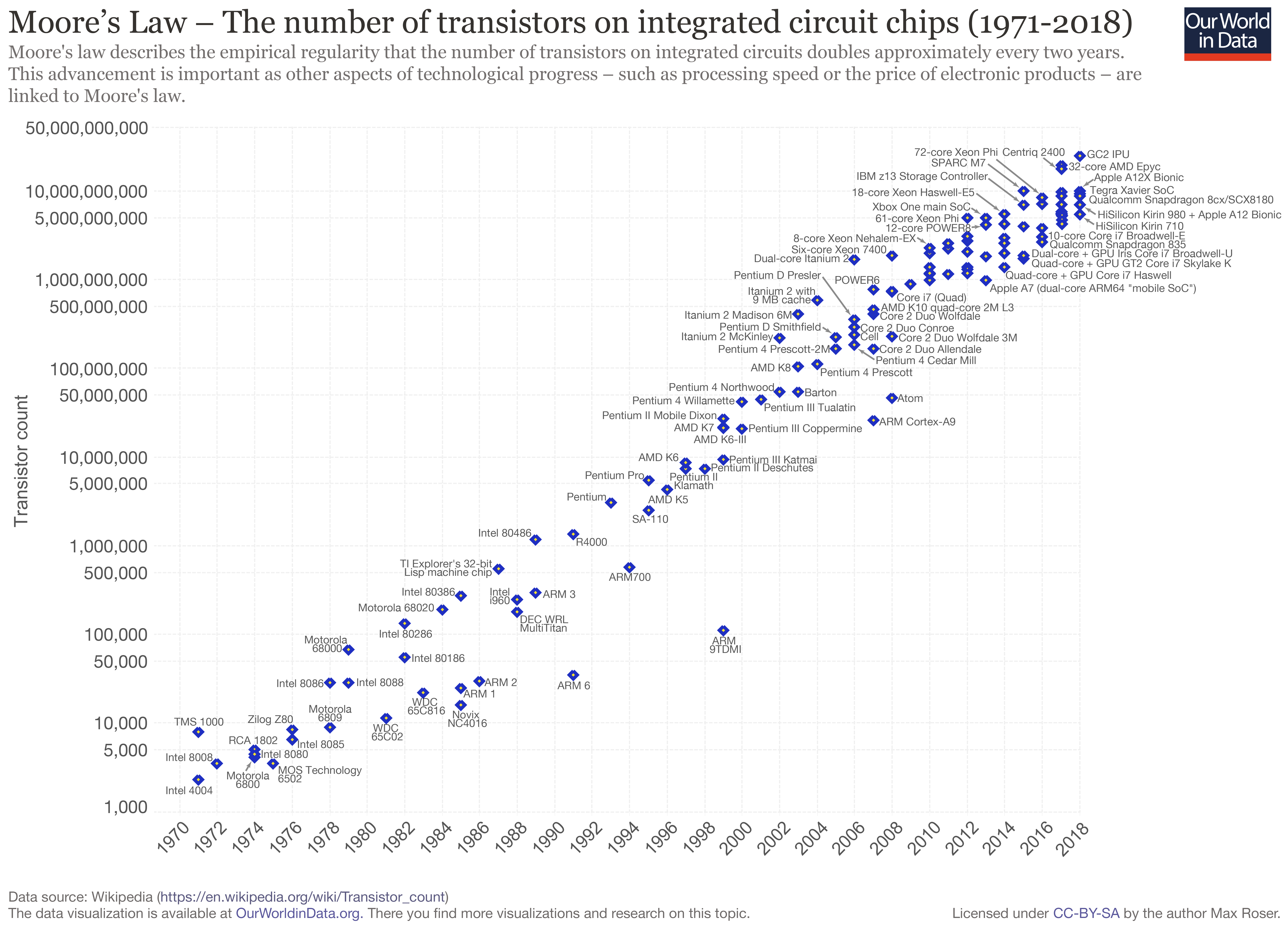
Fig. 18 Figure: Moore’s law. From Wikipedia, Creative Commons license.¶

The TOP500 list¶

The TOP500 list is, as the name suggests, is the list of 500 most powerful computers in the world. The first listing was done in June 1993 and the the list is updated twice a year, June and November. Currently (Nov. 2020), China has 212 systems on the list, the USA is the second with 113, and Japan the third with 34 systems. Canada has 12. Continent-wise top countries: Asia: China (overall #1 in terms of the number of systems), North America: USA (overall #2), Europe: Germany (#4), South America: Brazil (#12), Africa: Morocco (#27), Australia: Australia (#23).

Caveat: That a given country has a large number of systems on the list does not say anything about the access to those resources. For an individual researcher what matters is the ease of access and that is handled differently in each of the countries. In addition, countries and groups of countries have allocation modes that give preference to certain projects, that is, in the same style as grants. For example, In Canada Compute Canada/Calcul Canada has the normal allocation that is very easily accessible to researchers and a separate National Resource Allocation Competition which requires separate application and grants priority allocations to some systems and resources. In Europe, there is PRACE (Partnership for Advanced Computing in Europe). It has a pan-European competition for resource allocation.

Computing power now and in the past¶

After discussing the TOP500, it would be interesting to make a qualitative comparison to get a better idea what kind of computing power we all have in our hands. Try to find information on the computational power of

1990’s suprecomputer
Your laptop
Android phone
Gaming workstation

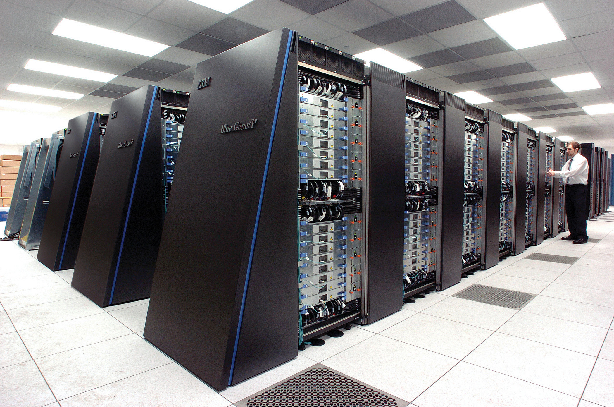
Fig. 19 IBM Blue Gene P. The Blue Gene family of computers were among the most powerful systems until to about 2015. Since then, IBM appears to have stopped the development. The Blue Gene/P that is in the figure was a 2nd generation Blue Gene computer. In terms of numbers, the processors on the Blue Gene/P were of IBM’s PowerPC type. A variant of the PowerPC chip was used in Macs before Apple switched to Intel processors in 2005. The Blue Gene/P used 850 GHz PowerPC450 processors. Figure: Wikipedia.¶

Distributed computing / cloud computing / citizen science¶

Distributed computing in its many forms has lead to very interesting projects including so-called citizen science in which individual people donate the idle time on their computer for research purposes.

Terminology: Double precision vs single precision¶

Single precision: 32 bit. Data type is called single. A floating point number is represented using 32 bits: 1 bit for the sign, 8 bits for the exponent and 23 bits for the mantissa. This means that the range of numbers is \(2^{-126}-2^{127}\) or \(\approx 1.18\times 10^{-38}-3.40\times 10^{38}\) (single precision)
Double precision: 64 bit. Data type is called double. A floating point number is represented using 64 bits: 1 bit for the sign, 11 bits for the exponent and 52 bits for the mantissa. The range of numbers is \(2^{-1022}-2^{1023}\).
Special cases: overflow, not-a-number, subnormal number

Most simulation software allow for compilaion in either single or double precision.

More:

IEEE Standard for Floating Point Numbers

We can also get that information from Python and Jupyter:

import sys

print("Smallest positive normalized float:", sys.float_info.min)
print("Largest float:", sys.float_info.max)
print("Float information:",sys.float_info)

Smallest positive normalized float: 2.2250738585072014e-308
Largest float: 1.7976931348623157e+308
Float information: sys.float_info(max=1.7976931348623157e+308, max_exp=1024, max_10_exp=308, min=2.2250738585072014e-308, min_exp=-1021, min_10_exp=-307, dig=15, mant_dig=53, epsilon=2.220446049250313e-16, radix=2, rounds=1)

# Need help on floats?

help(sys.float_info)

Help on float_info object:

class float_info(builtins.tuple)
 |  float_info(iterable=(), /)
 |  
 |  sys.float_info
 |  
 |  A named tuple holding information about the float type. It contains low level
 |  information about the precision and internal representation. Please study
 |  your system's :file:`float.h` for more information.
 |  
 |  Method resolution order:
 |      float_info
 |      builtins.tuple
 |      builtins.object
 |  
 |  Methods defined here:
 |  
 |  __reduce__(...)
 |      Helper for pickle.
 |  
 |  __repr__(self, /)
 |      Return repr(self).
 |  
 |  ----------------------------------------------------------------------
 |  Static methods defined here:
 |  
 |  __new__(*args, **kwargs) from builtins.type
 |      Create and return a new object.  See help(type) for accurate signature.
 |  
 |  ----------------------------------------------------------------------
 |  Data descriptors defined here:
 |  
 |  dig
 |      DBL_DIG -- digits
 |  
 |  epsilon
 |      DBL_EPSILON -- Difference between 1 and the next representable float
 |  
 |  mant_dig
 |      DBL_MANT_DIG -- mantissa digits
 |  
 |  max
 |      DBL_MAX -- maximum representable finite float
 |  
 |  max_10_exp
 |      DBL_MAX_10_EXP -- maximum int e such that 10**e is representable
 |  
 |  max_exp
 |      DBL_MAX_EXP -- maximum int e such that radix**(e-1) is representable
 |  
 |  min
 |      DBL_MIN -- Minimum positive normalized float
 |  
 |  min_10_exp
 |      DBL_MIN_10_EXP -- minimum int e such that 10**e is a normalized
 |  
 |  min_exp
 |      DBL_MIN_EXP -- minimum int e such that radix**(e-1) is a normalized float
 |  
 |  radix
 |      FLT_RADIX -- radix of exponent
 |  
 |  rounds
 |      FLT_ROUNDS -- rounding mode
 |  
 |  ----------------------------------------------------------------------
 |  Data and other attributes defined here:
 |  
 |  n_fields = 11
 |  
 |  n_sequence_fields = 11
 |  
 |  n_unnamed_fields = 0
 |  
 |  ----------------------------------------------------------------------
 |  Methods inherited from builtins.tuple:
 |  
 |  __add__(self, value, /)
 |      Return self+value.
 |  
 |  __contains__(self, key, /)
 |      Return key in self.
 |  
 |  __eq__(self, value, /)
 |      Return self==value.
 |  
 |  __ge__(self, value, /)
 |      Return self>=value.
 |  
 |  __getattribute__(self, name, /)
 |      Return getattr(self, name).
 |  
 |  __getitem__(self, key, /)
 |      Return self[key].
 |  
 |  __getnewargs__(self, /)
 |  
 |  __gt__(self, value, /)
 |      Return self>value.
 |  
 |  __hash__(self, /)
 |      Return hash(self).
 |  
 |  __iter__(self, /)
 |      Implement iter(self).
 |  
 |  __le__(self, value, /)
 |      Return self<=value.
 |  
 |  __len__(self, /)
 |      Return len(self).
 |  
 |  __lt__(self, value, /)
 |      Return self<value.
 |  
 |  __mul__(self, value, /)
 |      Return self*value.
 |  
 |  __ne__(self, value, /)
 |      Return self!=value.
 |  
 |  __rmul__(self, value, /)
 |      Return value*self.
 |  
 |  count(self, value, /)
 |      Return number of occurrences of value.
 |  
 |  index(self, value, start=0, stop=9223372036854775807, /)
 |      Return first index of value.
 |      
 |      Raises ValueError if the value is not present.

Scientific Computing

Background on computers, computing and High Performance Computing

Contents